Navier-Stokes equation and fluid simulation on CUDA
Note: if you are reading the Habr from a mobile device, and you don’t see the formulas, use the full version of the site
Navier-Stokes equation for an incompressible fluid
partial bf vecu over partialt=−( bf vecu cdot nabla) bf vecu−1 over rho nabla bfp+ nu nabla2 bf vecu+ bf vecF
I think everyone at least once heard about this equation, some, perhaps even analytically solved its particular cases, but in general terms this problem remains unresolved until now. Of course, we do not set the goal of solving the millennium problem in this article, however we can still apply the iterative method to it. But for starters, let's look at the notation in this formula.
Conventionally, the Navier-Stokes equation can be divided into five parts:
- partial bf vecu over partialt - indicates the acceleration at a time (we will consider it for each particle in our simulation).
- −( bf vecu cdot nabla) bf vecu - the movement of fluid in space.
- −1 over rho nabla bfp Is the pressure exerted on the particle (here rho - fluid density coefficient).
- nu nabla2 bf vecu - viscosity of the medium (the larger it is, the stronger the liquid resists the force applied to its part), nu - viscosity coefficient).
- bf vecF - external forces that we apply to the fluid (in our case, the force will play a very specific role - it will reflect the actions performed by the user.
Also, since we will consider the case of an incompressible and homogeneous fluid, we have another equation: nabla cdot bf vecu=0 . The energy in the environment is constant, does not go anywhere, does not come from anywhere.
It will be wrong to deprive all readers who are not familiar with vector analysis , so at the same time and briefly go through all the operators that are present in the equation (however, I highly recommend recalling what the derivative, differential and vector are, since they are the basis of all that what will be discussed below).
We start with the nabla operator, which is such a vector (in our case, it will be two-component, since we will model the liquid in two-dimensional space):
nabla= beginpmatrix partial over partialx, partial over partialy endpmatrix
The nabla operator is a vector differential operator and can be applied both to a scalar function and to a vector one. In the case of a scalar, we get the gradient of the function (the vector of its partial derivatives), and in the case of a vector, the sum of the partial derivatives along the axes. The main feature of this operator is that through it you can express the main operations of vector analysis - grad ( gradient ), div ( divergence ), rot ( rotor ) and nabla2 ( Laplace operator ). It is worth noting immediately that the expression ( bf vecu cdot nabla) bf vecu not tantamount to ( nabla cdot bf vecu) bf vecu - the nabla operator does not have commutativity.
As we will see later, these expressions are noticeably simplified when moving to a discrete space in which we will carry out all the calculations, so do not be alarmed if at the moment you are not very clear what to do with all this. Having divided the task into several parts, we will successively solve each of them and present all this in the form of the sequential application of several functions to our environment.
Numerical solution of the Navier-Stokes equation
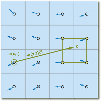
To represent our fluid in the program, we need to get a mathematical representation of the state of each fluid particle at an arbitrary point in time. The most convenient method for this is to create a vector field of particles storing their state in the form of a coordinate plane:

In each cell of our two-dimensional array, we will store the particle velocity at a time t: bf vecu=u( bf vecx,t), bf vecx= beginpmatrixx,y endpmatrix , and the distance between particles is denoted by deltax and deltay respectively. In the code, it will be enough for us to change the speed value each iteration, solving a set of several equations.
Now we express the gradient, divergence and the Laplace operator taking into account our coordinate grid ( i,j - indices in the array, bf vecu(x), vecu(y) - taking the corresponding components from the vector):
| Operator | Definition | Discrete Analog |
| grad | nabla bfp= beginpmatrix partial bfp over partialx, partial bfp over partialy endpmatrix | pi+1,j−pi−1,j over2 deltax,pi,j+1−pi,j−1 over2 deltay |
| div | nabla cdot bf vecu= partialu over partialx+ partialu over partialy | vecu(x)i+1,j− vecu(x)i−1,j over2 deltax+ vecu(y)i,j+1− vecu(y)i,j−1 over2 deltay |
| bf Delta | bf nabla2p= partial2p over partialx2+ partial2p over partialy2 | pi+1,j−2pi,j+pi−1,j over( deltax)2+pi,j+1−2pi,j+pi,j−1 over( deltay)2 |
| rot | bf nabla times vecu= partial vecu over partialy− partial vecu over partialx | vecu(y)i,j+1− vecu(y)i,j−1 over2 deltay− vecu(x)i+1,j− vecu(x)i−1,j over2 deltax |
We can further simplify the discrete formulas of vector operators if we assume that deltax= deltay=1 . This assumption will not greatly affect the accuracy of the algorithm, however, it reduces the number of operations per iteration, and generally makes expressions more pleasant to the eye.
Particle movement
These statements work only if we can find the nearest particles relative to the one under consideration at the moment. In order to negate all possible costs associated with the search for such, we will not track their movement, but rather where the particles come from at the beginning of the iteration by projecting the trajectory of movement backward in time (in other words, subtract the velocity vector times the time change from current position). Using this technique for each element of the array, we will be sure that any particle will have “neighbors”:
Putting that q - an array element that stores the state of the particle, we obtain the following formula for calculating its state over time deltat (we believe that all the necessary parameters in the form of acceleration and pressure have already been calculated):
q( vec bfx,t+ deltat)=q( bf vecx− bf vecu deltat,t)
We note immediately that for sufficiently small deltat and we can never go beyond the limits of the cell, so it is very important to choose the right momentum that the user will give to the particles.
In order to avoid loss of accuracy in the case of a projection at the cell boundary or in the case of non-integer coordinates, we will carry out bilinear interpolation of the states of the four nearest particles and take it as the true value at the point. In principle, such a method will practically not reduce the accuracy of the simulation, and at the same time it is quite simple to implement, so we will use it.
Viscosity
Each liquid has a certain viscosity, the ability to prevent the influence of external forces on its parts (honey and water will be a good example, in some cases their viscosity coefficients differ by an order of magnitude). Viscosity directly affects the acceleration acquired by the liquid, and can be expressed by the formula below, if for brevity we omit other terms for a while:
partial vec bfu over partialt= nu nabla2 bf vecu
. In this case, the iterative equation for speed takes the following form:
u( bf vecx,t+ deltat)=u( bf vecx,t)+ nu deltat nabla2 bf vecu
We will slightly transform this equality, bringing it to the form bfA vecx= vecb (standard form of a system of linear equations):
( bfI− nu deltat nabla2)u( bf vecx,t+ deltat)=u( bf vecx,t)
Where bfI Is the identity matrix. We need such transformations in order to later apply the Jacobi method for solving several similar systems of equations. We will also discuss it later.
External forces
The simplest step of the algorithm is the application of external forces to the medium. For the user, this will be reflected in the form of clicks on the screen with the mouse or its movement. External force can be described by the following formula, which we apply for each element of the matrix ( vec bfG - momentum vector xp,yp - mouse position x,y - coordinates of the current cell, r - radius of action, scaling parameter):
vec bfF= vec bfG deltat bfexp left(−(x−xp)2+(y−yp)2 overr right)
An impulse vector can be easily calculated as the difference between the previous position of the mouse and the current one (if there was one), and here you can still be creative. It is in this part of the algorithm that we can introduce the addition of colors to a liquid, its illumination, etc. External forces can also include gravity and temperature, and although it is not difficult to implement such parameters, we will not consider them in this article.
Pressure
The pressure in the Navier-Stokes equation is the force that prevents particles from filling up all the space available to them after applying any external force to them. Immediately, its calculation is very difficult, but our problem can be greatly simplified by applying the Helmholtz decomposition theorem .
Call bf vecW vector field obtained after calculating displacement, external forces and viscosity. It will have nonzero divergence, which contradicts the condition of fluid incompressibility ( nabla cdot bf vecu=0 ), and in order to fix this, it is necessary to calculate the pressure. According to the Helmholtz decomposition theorem, bf vecW can be represented as the sum of two fields:
bf vecW= vecu+ nablap
Where bfu - this is the vector field we are looking for with zero divergence. No proof of this equality will be given in this article, however at the end you can find a link with a detailed explanation. We can apply the nabla operator to both sides of the expression to get the following formula for calculating the scalar pressure field:
nabla cdot bf vecW= nabla cdot( vecu+ nablap)= nabla cdot vecu+ nabla2p= nabla2p
The expression written above is the Poisson equation for pressure. We can also solve it by the aforementioned Jacobi method, and thereby find the last unknown variable in the Navier-Stokes equation. In principle, systems of linear equations can be solved in a variety of different and sophisticated ways, but we will still dwell on the simplest of them, so as not to further burden this article.
Boundary and initial conditions
Any differential equation modeled on a finite domain requires correctly specified initial or boundary conditions, otherwise we are very likely to get a physically incorrect result. Boundary conditions are established to control the behavior of the fluid near the edges of the grid, and the initial conditions specify the parameters that the particles have at the time the program starts.
The initial conditions will be very simple - initially the fluid is stationary (particle velocity is zero), and the pressure is also zero. The boundary conditions will be set for speed and pressure by the given formulas:
bf vecu0,j+ bf vecu1,j over2 deltay=0, bf vecui,0+ bf vecui,1 over2 deltax=0
bfp0,j− bfp1,j over deltax=0, bfpi,0− bfpi,1 over deltay=0
Thus, the velocity of the particles at the edges will be opposite to the velocity at the edges (thereby they will repel from the edge), and the pressure is equal to the value immediately next to the boundary. These operations should be applied to all bounding elements of the array (for example, there is a grid size N timesM , then we apply the algorithm for cells marked in blue in the figure):

Dye
With what we have now, you can already come up with a lot of interesting things. For example, to realize the spread of dye in a liquid. To do this, we just need to maintain another scalar field, which would be responsible for the amount of paint at each point of the simulation. The formula for updating the dye is very similar to speed, and is expressed as:
partiald over partialt=−( vec bfu cdot nabla)d+ gamma nabla2d+S
In the formula S responsible for replenishing the area with a dye (possibly depending on where the user clicks), d directly is the amount of dye at the point, and gamma - diffusion coefficient. Solving it is not difficult, since all the basic work on the derivation of formulas has already been carried out, and it is enough to make a few substitutions. Paint can be implemented in the code as a color in the RGB format, and in this case the task is reduced to operations with several real values.
Vorticity
The vorticity equation is not a direct part of the Navier-Stokes equation, but it is an important parameter for a plausible simulation of the motion of a dye in a liquid. Due to the fact that we produce the algorithm on a discrete field, as well as due to losses in the accuracy of the values of the floating point, this effect is lost, and therefore we need to restore it by applying additional force to each point in space. The vector of this force is designated as bf vecT and is determined by the following formulas:
bf omega= nabla times vecu
vec eta= nabla| omega|
bf vec psi= vec eta over| vec eta|
bf vecT= epsilon( vec psi times omega) deltax
omega there is the result of applying the rotor to the velocity vector (its definition is given at the beginning of the article), vec eta - gradient of the scalar field of absolute values omega . vec psi represents a normalized vector vec eta , but epsilon Is a constant that controls how large the vortices in our fluid will be.
Jacobi method for solving systems of linear equations
In analyzing the Navier-Stokes equation, we came up with two systems of equations - one for viscosity, the other for pressure. They can be solved by an iterative algorithm, which can be described by the following iterative formula:
x(k+1)i,j=x(k)i−1,j+x(k)i+1,j+x(k)i,j−1+x(k)i,j+1+ alphabi,j over beta
For us x - array elements representing a scalar or vector field. k - the iteration number, we can adjust it in order to increase the accuracy of the calculation or vice versa to reduce it and increase productivity.
To calculate the viscosity we substitute: x=b= bf vecu , alpha=1 over nu deltat , beta=4+ alpha , here is the parameter beta - the sum of the weights. Thus, we need to store at least two vector velocity fields in order to independently read the values of one field and write them to another. On average, to calculate the velocity field using the Jacobi method, it is necessary to carry out 20-50 iterations, which is quite a lot if we were to perform calculations on the CPU.
For the pressure equation, we make the following substitution: x=p , b= nabla bf cdot vecW , a l p h a = - 1 , b e t a = 4 . As a result, we get the value p i , j d e l t a t at the point. But since it is used only for calculating the gradient subtracted from the velocity field, additional transformations can be omitted. For a pressure field, it is best to perform 40-80 iterations, because with smaller numbers the discrepancy becomes noticeable.
Algorithm implementation
We will implement the algorithm in C ++, we also need the Cuda Toolkit (you can read how to install it on the Nvidia website), as well as SFML . We need CUDA to parallelize the algorithm, and SFML will only be used to create a window and display a picture on the screen (In principle, this can be written in OpenGL, but the difference in performance will be insignificant, but the code will increase by another 200 lines).
Cuda toolkit
First, we'll talk a bit about how to use the Cuda Toolkit to parallelize tasks. A more detailed guide is provided by Nvidia itself, so here we restrict ourselves to only the most necessary. It is also assumed that you were able to install the compiler, and you were able to build a test project without errors.
To create a function that runs on the GPU, you first need to declare how many cores we want to use, and how many blocks of cores to allocate. For this, the Cuda Toolkit provides us with a special structure - dim3 , by default setting all its x, y, z values to 1. By specifying it as an argument when calling the function, we can control the number of allocated kernels. Since we are working with a two-dimensional array, we need to set only two fields in the constructor: x and y :
dim3 threadsPerBlock(x_threads, y_threads); dim3 numBlocks(size_x / x_threads, y_size / y_threads);
where size_x and size_y are the size of the array being processed. The signature and function call are as follows (triple angle brackets are processed by the Cuda compiler):
void __global__ deviceFunction(); // declare deviceFunction<<<numBlocks, threadsPerBlock>>>(); // call from host
In the function itself, you can restore the indices of a two-dimensional array through the block number and the kernel number in this block using the following formula:
int x = blockIdx.x * blockDim.x + threadIdx.x; int y = blockIdx.y * blockDim.y + threadIdx.y;
It should be noted that the function executed on the video card must be marked with the __global__ tag, and also return void , so most often the results of the calculations are written to the array passed as an argument and pre-allocated in the memory of the video card.
The functions CudaMalloc and CudaFree are responsible for freeing and allocating memory on the video card. We can operate with pointers to the memory area that they return, but we cannot access the data from the main code. The easiest way to return the results of calculations is to use cudaMemcpy , similar to the standard memcpy , but able to copy data from a video card to main memory and vice versa.
SFML and window render
Armed with all this knowledge, we can finally move on to writing code directly. To start, let's create the main.cpp file and place all the auxiliary code for the window render there:
#include <SFML/Graphics.hpp> #include <chrono> #include <cstdlib> #include <cmath> //SFML REQUIRED TO LAUNCH THIS CODE #define SCALE 2 #define WINDOW_WIDTH 1280 #define WINDOW_HEIGHT 720 #define FIELD_WIDTH WINDOW_WIDTH / SCALE #define FIELD_HEIGHT WINDOW_HEIGHT / SCALE static struct Config { float velocityDiffusion; float pressure; float vorticity; float colorDiffusion; float densityDiffusion; float forceScale; float bloomIntense; int radius; bool bloomEnabled; } config; void setConfig(float vDiffusion = 0.8f, float pressure = 1.5f, float vorticity = 50.0f, float cDiffuion = 0.8f, float dDiffuion = 1.2f, float force = 1000.0f, float bloomIntense = 25000.0f, int radius = 100, bool bloom = true); void computeField(uint8_t* result, float dt, int x1pos = -1, int y1pos = -1, int x2pos = -1, int y2pos = -1, bool isPressed = false); void cudaInit(size_t xSize, size_t ySize); void cudaExit(); int main() { cudaInit(FIELD_WIDTH, FIELD_HEIGHT); srand(time(NULL)); sf::RenderWindow window(sf::VideoMode(WINDOW_WIDTH, WINDOW_HEIGHT), ""); auto start = std::chrono::system_clock::now(); auto end = std::chrono::system_clock::now(); sf::Texture texture; sf::Sprite sprite; std::vector<sf::Uint8> pixelBuffer(FIELD_WIDTH * FIELD_HEIGHT * 4); texture.create(FIELD_WIDTH, FIELD_HEIGHT); sf::Vector2i mpos1 = { -1, -1 }, mpos2 = { -1, -1 }; bool isPressed = false; bool isPaused = false; while (window.isOpen()) { end = std::chrono::system_clock::now(); std::chrono::duration<float> diff = end - start; window.setTitle("Fluid simulator " + std::to_string(int(1.0f / diff.count())) + " fps"); start = end; window.clear(sf::Color::White); sf::Event event; while (window.pollEvent(event)) { if (event.type == sf::Event::Closed) window.close(); if (event.type == sf::Event::MouseButtonPressed) { if (event.mouseButton.button == sf::Mouse::Button::Left) { mpos1 = { event.mouseButton.x, event.mouseButton.y }; mpos1 /= SCALE; isPressed = true; } else { isPaused = !isPaused; } } if (event.type == sf::Event::MouseButtonReleased) { isPressed = false; } if (event.type == sf::Event::MouseMoved) { std::swap(mpos1, mpos2); mpos2 = { event.mouseMove.x, event.mouseMove.y }; mpos2 /= SCALE; } } float dt = 0.02f; if (!isPaused) computeField(pixelBuffer.data(), dt, mpos1.x, mpos1.y, mpos2.x, mpos2.y, isPressed); texture.update(pixelBuffer.data()); sprite.setTexture(texture); sprite.setScale({ SCALE, SCALE }); window.draw(sprite); window.display(); } cudaExit(); return 0; }
line at the beginning of the main function
std::vector<sf::Uint8> pixelBuffer(FIELD_WIDTH * FIELD_HEIGHT * 4);
creates an RGBA image in the form of a one-dimensional array with a constant length. We will pass it along with other parameters (mouse position, difference between frames) to the computeField function. The latter, as well as several other functions, are declared in kernel.cu and call the code executed on the GPU. You can find documentation on any of the functions on the SFML website, nothing super interesting happens in the file code, so we won’t stop there for long.
GPU Computing
To start writing code under gpu, first create a kernel.cu file and define several auxiliary classes in it: Color3f, Vec2, Config, SystemConfig :
struct Vec2 { float x = 0.0, y = 0.0; __device__ Vec2 operator-(Vec2 other) { Vec2 res; res.x = this->x - other.x; res.y = this->y - other.y; return res; } __device__ Vec2 operator+(Vec2 other) { Vec2 res; res.x = this->x + other.x; res.y = this->y + other.y; return res; } __device__ Vec2 operator*(float d) { Vec2 res; res.x = this->x * d; res.y = this->y * d; return res; } }; struct Color3f { float R = 0.0f; float G = 0.0f; float B = 0.0f; __host__ __device__ Color3f operator+ (Color3f other) { Color3f res; res.R = this->R + other.R; res.G = this->G + other.G; res.B = this->B + other.B; return res; } __host__ __device__ Color3f operator* (float d) { Color3f res; res.R = this->R * d; res.G = this->G * d; res.B = this->B * d; return res; } }; struct Particle { Vec2 u; // velocity Color3f color; }; static struct Config { float velocityDiffusion; float pressure; float vorticity; float colorDiffusion; float densityDiffusion; float forceScale; float bloomIntense; int radius; bool bloomEnabled; } config; static struct SystemConfig { int velocityIterations = 20; int pressureIterations = 40; int xThreads = 64; int yThreads = 1; } sConfig; void setConfig( float vDiffusion = 0.8f, float pressure = 1.5f, float vorticity = 50.0f, float cDiffuion = 0.8f, float dDiffuion = 1.2f, float force = 5000.0f, float bloomIntense = 25000.0f, int radius = 500, bool bloom = true ) { config.velocityDiffusion = vDiffusion; config.pressure = pressure; config.vorticity = vorticity; config.colorDiffusion = cDiffuion; config.densityDiffusion = dDiffuion; config.forceScale = force; config.bloomIntense = bloomIntense; config.radius = radius; config.bloomEnabled = bloom; } static const int colorArraySize = 7; Color3f colorArray[colorArraySize]; static Particle* newField; static Particle* oldField; static uint8_t* colorField; static size_t xSize, ySize; static float* pressureOld; static float* pressureNew; static float* vorticityField; static Color3f currentColor; static float elapsedTime = 0.0f; static float timeSincePress = 0.0f; static float bloomIntense; int lastXpos = -1, lastYpos = -1;
The __host__ attribute in front of the method name means that the code can be executed on the CPU, __device__ , on the contrary, requires the compiler to compile code under the GPU. The code declares primitives for working with two-component vectors, color, configs with parameters that can be changed in runtime, as well as several static pointers to arrays, which we will use as buffers for calculations.
cudaInit and cudaExit are also defined quite trivially:
void cudaInit(size_t x, size_t y) { setConfig(); colorArray[0] = { 1.0f, 0.0f, 0.0f }; colorArray[1] = { 0.0f, 1.0f, 0.0f }; colorArray[2] = { 1.0f, 0.0f, 1.0f }; colorArray[3] = { 1.0f, 1.0f, 0.0f }; colorArray[4] = { 0.0f, 1.0f, 1.0f }; colorArray[5] = { 1.0f, 0.0f, 1.0f }; colorArray[6] = { 1.0f, 0.5f, 0.3f }; int idx = rand() % colorArraySize; currentColor = colorArray[idx]; xSize = x, ySize = y; cudaSetDevice(0); cudaMalloc(&colorField, xSize * ySize * 4 * sizeof(uint8_t)); cudaMalloc(&oldField, xSize * ySize * sizeof(Particle)); cudaMalloc(&newField, xSize * ySize * sizeof(Particle)); cudaMalloc(&pressureOld, xSize * ySize * sizeof(float)); cudaMalloc(&pressureNew, xSize * ySize * sizeof(float)); cudaMalloc(&vorticityField, xSize * ySize * sizeof(float)); } void cudaExit() { cudaFree(colorField); cudaFree(oldField); cudaFree(newField); cudaFree(pressureOld); cudaFree(pressureNew); cudaFree(vorticityField); }
In the initialization function, we allocate memory for two-dimensional arrays, specify an array of colors that we will use to paint the liquid, and also set the default values in the config. In cudaExit, we just free all buffers. As paradoxical as it sounds, for storing two-dimensional arrays, it is most advantageous to use one-dimensional arrays, access to which will be carried out with the following expression:
array[y * size_x + x]; // equals to array[y][x]
We begin the implementation of the direct algorithm with the particle movement function. The fields oldField and newField (the field where the data come from and where they are written to), the size of the array, as well as the time delta and density coefficient (used to accelerate the dissolution of the dye in the liquid and make the medium not very sensitive to advect, are transferred to advect user actions). The bilinear interpolation function is implemented in a classical way by calculating intermediate values:
// interpolates quantity of grid cells __device__ Particle interpolate(Vec2 v, Particle* field, size_t xSize, size_t ySize) { float x1 = (int)vx; float y1 = (int)vy; float x2 = (int)vx + 1; float y2 = (int)vy + 1; Particle q1, q2, q3, q4; #define CLAMP(val, minv, maxv) min(maxv, max(minv, val)) #define SET(Q, x, y) Q = field[int(CLAMP(y, 0.0f, ySize - 1.0f)) * xSize + int(CLAMP(x, 0.0f, xSize - 1.0f))] SET(q1, x1, y1); SET(q2, x1, y2); SET(q3, x2, y1); SET(q4, x2, y2); #undef SET #undef CLAMP float t1 = (x2 - vx) / (x2 - x1); float t2 = (vx - x1) / (x2 - x1); Vec2 f1 = q1.u * t1 + q3.u * t2; Vec2 f2 = q2.u * t1 + q4.u * t2; Color3f C1 = q2.color * t1 + q4.color * t2; Color3f C2 = q2.color * t1 + q4.color * t2; float t3 = (y2 - vy) / (y2 - y1); float t4 = (vy - y1) / (y2 - y1); Particle res; res.u = f1 * t3 + f2 * t4; res.color = C1 * t3 + C2 * t4; return res; } // adds quantity to particles using bilinear interpolation __global__ void advect(Particle* newField, Particle* oldField, size_t xSize, size_t ySize, float dDiffusion, float dt) { int x = blockIdx.x * blockDim.x + threadIdx.x; int y = blockIdx.y * blockDim.y + threadIdx.y; float decay = 1.0f / (1.0f + dDiffusion * dt); Vec2 pos = { x * 1.0f, y * 1.0f }; Particle& Pold = oldField[y * xSize + x]; // find new particle tracing where it came from Particle p = interpolate(pos - Pold.u * dt, oldField, xSize, ySize); pu = pu * decay; p.color = p.color * decay; newField[y * xSize + x] = p; }
It was decided to divide the viscosity diffusion function into several parts: computeDiffusion is called from the main code, which calls diffuse and computeColor a predetermined number of times, and then swaps the array from where we take the data and the one where we write it. This is the easiest way to implement parallel data processing, but we are spending twice as much memory.
Both functions cause variations of the Jacobi method. The body of jacobiColor and jacobiVelocity immediately checks that the current elements are not on the border - in this case, we must set them in accordance with the formulas described in the Boundary and initial conditions section.
// performs iteration of jacobi method on color grid field __device__ Color3f jacobiColor(Particle* colorField, size_t xSize, size_t ySize, Vec2 pos, Color3f B, float alpha, float beta) { Color3f xU, xD, xL, xR, res; int x = pos.x; int y = pos.y; #define SET(P, x, y) if (x < xSize && x >= 0 && y < ySize && y >= 0) P = colorField[int(y) * xSize + int(x)] SET(xU, x, y - 1).color; SET(xD, x, y + 1).color; SET(xL, x - 1, y).color; SET(xR, x + 1, y).color; #undef SET res = (xU + xD + xL + xR + B * alpha) * (1.0f / beta); return res; } // calculates color field diffusion __global__ void computeColor(Particle* newField, Particle* oldField, size_t xSize, size_t ySize, float cDiffusion, float dt) { int x = blockIdx.x * blockDim.x + threadIdx.x; int y = blockIdx.y * blockDim.y + threadIdx.y; Vec2 pos = { x * 1.0f, y * 1.0f }; Color3f c = oldField[y * xSize + x].color; float alpha = cDiffusion * cDiffusion / dt; float beta = 4.0f + alpha; // perfom one iteration of jacobi method (diffuse method should be called 20-50 times per cell) newField[y * xSize + x].color = jacobiColor(oldField, xSize, ySize, pos, c, alpha, beta); } // performs iteration of jacobi method on velocity grid field __device__ Vec2 jacobiVelocity(Particle* field, size_t xSize, size_t ySize, Vec2 v, Vec2 B, float alpha, float beta) { Vec2 vU = B * -1.0f, vD = B * -1.0f, vR = B * -1.0f, vL = B * -1.0f; #define SET(U, x, y) if (x < xSize && x >= 0 && y < ySize && y >= 0) U = field[int(y) * xSize + int(x)].u SET(vU, vx, vy - 1); SET(vD, vx, vy + 1); SET(vL, vx - 1, vy); SET(vR, vx + 1, vy); #undef SET v = (vU + vD + vL + vR + B * alpha) * (1.0f / beta); return v; } // calculates nonzero divergency velocity field u __global__ void diffuse(Particle* newField, Particle* oldField, size_t xSize, size_t ySize, float vDiffusion, float dt) { int x = blockIdx.x * blockDim.x + threadIdx.x; int y = blockIdx.y * blockDim.y + threadIdx.y; Vec2 pos = { x * 1.0f, y * 1.0f }; Vec2 u = oldField[y * xSize + x].u; // perfoms one iteration of jacobi method (diffuse method should be called 20-50 times per cell) float alpha = vDiffusion * vDiffusion / dt; float beta = 4.0f + alpha; newField[y * xSize + x].u = jacobiVelocity(oldField, xSize, ySize, pos, u, alpha, beta); } // performs several iterations over velocity and color fields void computeDiffusion(dim3 numBlocks, dim3 threadsPerBlock, float dt) { // diffuse velocity and color for (int i = 0; i < sConfig.velocityIterations; i++) { diffuse<<<numBlocks, threadsPerBlock>>>(newField, oldField, xSize, ySize, config.velocityDiffusion, dt); computeColor<<<numBlocks, threadsPerBlock>>>(newField, oldField, xSize, ySize, config.colorDiffusion, dt); std::swap(newField, oldField); } }
The use of external force is implemented through a single function - applyForce , which takes as an argument the position of the mouse, the color of the dye, and also the radius of action. With its help, we can give speed to the particles, as well as paint them. The fraternal exponent allows you to make the area not too sharp, and at the same time quite clear in the specified radius.
// applies force and add color dye to the particle field __global__ void applyForce(Particle* field, size_t xSize, size_t ySize, Color3f color, Vec2 F, Vec2 pos, int r, float dt) { int x = blockIdx.x * blockDim.x + threadIdx.x; int y = blockIdx.y * blockDim.y + threadIdx.y; float e = expf((-(powf(x - pos.x, 2) + powf(y - pos.y, 2))) / r); Vec2 uF = F * dt * e; Particle& p = field[y * xSize + x]; pu = pu + uF; color = color * e + p.color; p.color.R = min(1.0f, color.R); p.color.G = min(1.0f, color.G); p.color.B = min(1.0f, color.B); }
The calculation of vorticity is already a more complex process, so we implement it in computeVorticity and applyVorticity , we also note that for them it is necessary to define two such vector operators as curl (rotor) and absGradient (gradient of absolute field values). To specify additional vortex effects, we multiply y component of the gradient vector on - 1 , and then normalize it by dividing by the length (without forgetting to check that the vector is nonzero):
// computes curl of velocity field __device__ float curl(Particle* field, size_t xSize, size_t ySize, int x, int y) { Vec2 C = field[int(y) * xSize + int(x)].u; #define SET(P, x, y) if (x < xSize && x >= 0 && y < ySize && y >= 0) P = field[int(y) * xSize + int(x)] float x1 = -Cx, x2 = -Cx, y1 = -Cy, y2 = -Cy; SET(x1, x + 1, y).ux; SET(x2, x - 1, y).ux; SET(y1, x, y + 1).uy; SET(y2, x, y - 1).uy; #undef SET float res = ((y1 - y2) - (x1 - x2)) * 0.5f; return res; } // computes absolute value gradient of vorticity field __device__ Vec2 absGradient(float* field, size_t xSize, size_t ySize, int x, int y) { float C = field[int(y) * xSize + int(x)]; #define SET(P, x, y) if (x < xSize && x >= 0 && y < ySize && y >= 0) P = field[int(y) * xSize + int(x)] float x1 = C, x2 = C, y1 = C, y2 = C; SET(x1, x + 1, y); SET(x2, x - 1, y); SET(y1, x, y + 1); SET(y2, x, y - 1); #undef SET Vec2 res = { (abs(x1) - abs(x2)) * 0.5f, (abs(y1) - abs(y2)) * 0.5f }; return res; } // computes vorticity field which should be passed to applyVorticity function __global__ void computeVorticity(float* vField, Particle* field, size_t xSize, size_t ySize) { int x = blockIdx.x * blockDim.x + threadIdx.x; int y = blockIdx.y * blockDim.y + threadIdx.y; vField[y * xSize + x] = curl(field, xSize, ySize, x, y); } // applies vorticity to velocity field __global__ void applyVorticity(Particle* newField, Particle* oldField, float* vField, size_t xSize, size_t ySize, float vorticity, float dt) { int x = blockIdx.x * blockDim.x + threadIdx.x; int y = blockIdx.y * blockDim.y + threadIdx.y; Particle& pOld = oldField[y * xSize + x]; Particle& pNew = newField[y * xSize + x]; Vec2 v = absGradient(vField, xSize, ySize, x, y); vy *= -1.0f; float length = sqrtf(vx * vx + vy * vy) + 1e-5f; Vec2 vNorm = v * (1.0f / length); Vec2 vF = vNorm * vField[y * xSize + x] * vorticity; pNew = pOld; pNew.u = pNew.u + vF * dt; }
The next step in the algorithm will be the calculation of the scalar pressure field and its projection on the velocity field. To do this, we need to implement 4 functions: divergency , which will consider the speed divergence, jacobiPressure , which implements the Jacobi method for pressure, and computePressure with computePressureImpl , which iterates field calculations:
// performs iteration of jacobi method on pressure grid field __device__ float jacobiPressure(float* pressureField, size_t xSize, size_t ySize, int x, int y, float B, float alpha, float beta) { float C = pressureField[int(y) * xSize + int(x)]; float xU = C, xD = C, xL = C, xR = C; #define SET(P, x, y) if (x < xSize && x >= 0 && y < ySize && y >= 0) P = pressureField[int(y) * xSize + int(x)] SET(xU, x, y - 1); SET(xD, x, y + 1); SET(xL, x - 1, y); SET(xR, x + 1, y); #undef SET float pressure = (xU + xD + xL + xR + alpha * B) * (1.0f / beta); return pressure; } // computes divergency of velocity field __device__ float divergency(Particle* field, size_t xSize, size_t ySize, int x, int y) { Particle& C = field[int(y) * xSize + int(x)]; float x1 = -1 * Cux, x2 = -1 * Cux, y1 = -1 * Cuy, y2 = -1 * Cuy; #define SET(P, x, y) if (x < xSize && x >= 0 && y < ySize && y >= 0) P = field[int(y) * xSize + int(x)] SET(x1, x + 1, y).ux; SET(x2, x - 1, y).ux; SET(y1, x, y + 1).uy; SET(y2, x, y - 1).uy; #undef SET return (x1 - x2 + y1 - y2) * 0.5f; } // performs iteration of jacobi method on pressure field __global__ void computePressureImpl(Particle* field, size_t xSize, size_t ySize, float* pNew, float* pOld, float pressure, float dt) { int x = blockIdx.x * blockDim.x + threadIdx.x; int y = blockIdx.y * blockDim.y + threadIdx.y; float div = divergency(field, xSize, ySize, x, y); float alpha = -1.0f * pressure * pressure; float beta = 4.0; pNew[y * xSize + x] = jacobiPressure(pOld, xSize, ySize, x, y, div, alpha, beta); } // performs several iterations over pressure field void computePressure(dim3 numBlocks, dim3 threadsPerBlock, float dt) { for (int i = 0; i < sConfig.pressureIterations; i++) { computePressureImpl<<<numBlocks, threadsPerBlock>>>(oldField, xSize, ySize, pressureNew, pressureOld, config.pressure, dt); std::swap(pressureOld, pressureNew); } }
The projection fits in two small functions - project and the gradient it calls for pressure. This can be said the last stage of our simulation algorithm:
// computes gradient of pressure field __device__ Vec2 gradient(float* field, size_t xSize, size_t ySize, int x, int y) { float C = field[y * xSize + x]; #define SET(P, x, y) if (x < xSize && x >= 0 && y < ySize && y >= 0) P = field[int(y) * xSize + int(x)] float x1 = C, x2 = C, y1 = C, y2 = C; SET(x1, x + 1, y); SET(x2, x - 1, y); SET(y1, x, y + 1); SET(y2, x, y - 1); #undef SET Vec2 res = { (x1 - x2) * 0.5f, (y1 - y2) * 0.5f }; return res; } // projects pressure field on velocity field __global__ void project(Particle* newField, size_t xSize, size_t ySize, float* pField) { int x = blockIdx.x * blockDim.x + threadIdx.x; int y = blockIdx.y * blockDim.y + threadIdx.y; Vec2& u = newField[y * xSize + x].u; u = u - gradient(pField, xSize, ySize, x, y); }
After the projection, we can safely proceed to rendering the image to the buffer and various post-effects. The paint function copies colors from the particle field to the RGBA array. The applyBloom function was also implemented, which highlights the liquid when the cursor is placed on it and the mouse button is pressed. From experience, this technique makes the picture more pleasant and interesting for the user's eyes, but it is not necessary at all.
In post-processing, you can also highlight places where the fluid has the highest speed, change color depending on the motion vector, add various effects, etc., but in our case we will limit ourselves to a kind of minimum, because even with it the images are very fascinating (especially in dynamics) :
// adds flashlight effect near the mouse position __global__ void applyBloom(uint8_t* colorField, size_t xSize, size_t ySize, int xpos, int ypos, float bloomIntense) { int x = blockIdx.x * blockDim.x + threadIdx.x; int y = blockIdx.y * blockDim.y + threadIdx.y; int pos = 4 * (y * xSize + x); float e = expf(-(powf(x - xpos, 2) + powf(y - ypos, 2)) * (1.0f / (bloomIntense + 1e-5f))); uint8_t R = colorField[pos + 0]; uint8_t G = colorField[pos + 1]; uint8_t B = colorField[pos + 2]; uint8_t maxval = max(R, max(G, B)); colorField[pos + 0] = min(255.0f, R + maxval * e); colorField[pos + 1] = min(255.0f, G + maxval * e); colorField[pos + 2] = min(255.0f, B + maxval * e); } // fills output image with corresponding color __global__ void paint(uint8_t* colorField, Particle* field, size_t xSize, size_t ySize) { int x = blockIdx.x * blockDim.x + threadIdx.x; int y = blockIdx.y * blockDim.y + threadIdx.y; float R = field[y * xSize + x].color.R; float G = field[y * xSize + x].color.G; float B = field[y * xSize + x].color.B; colorField[4 * (y * xSize + x) + 0] = min(255.0f, 255.0f * R); colorField[4 * (y * xSize + x) + 1] = min(255.0f, 255.0f * G); colorField[4 * (y * xSize + x) + 2] = min(255.0f, 255.0f * B); colorField[4 * (y * xSize + x) + 3] = 255; }
And in the end, we still have one main function that we call from main.cpp - computeField . It links together all the pieces of the algorithm, calling the code on the video card, and also copies the data from gpu to cpu. It also contains the calculation of the momentum vector and the choice of dye color, which we pass to applyForce :
// main function, calls vorticity -> diffusion -> force -> pressure -> project -> advect -> paint -> bloom void computeField(uint8_t* result, float dt, int x1pos, int y1pos, int x2pos, int y2pos, bool isPressed) { dim3 threadsPerBlock(sConfig.xThreads, sConfig.yThreads); dim3 numBlocks(xSize / threadsPerBlock.x, ySize / threadsPerBlock.y); // curls and vortisity computeVorticity<<<numBlocks, threadsPerBlock>>>(vorticityField, oldField, xSize, ySize); applyVorticity<<<numBlocks, threadsPerBlock>>>(newField, oldField, vorticityField, xSize, ySize, config.vorticity, dt); std::swap(oldField, newField); // diffuse velocity and color computeDiffusion(numBlocks, threadsPerBlock, dt); // apply force if (isPressed) { timeSincePress = 0.0f; elapsedTime += dt; // apply gradient to color int roundT = int(elapsedTime) % colorArraySize; int ceilT = int((elapsedTime) + 1) % colorArraySize; float w = elapsedTime - int(elapsedTime); currentColor = colorArray[roundT] * (1 - w) + colorArray[ceilT] * w; Vec2 F; float scale = config.forceScale; Fx = (x2pos - x1pos) * scale; Fy = (y2pos - y1pos) * scale; Vec2 pos = { x2pos * 1.0f, y2pos * 1.0f }; applyForce<<<numBlocks, threadsPerBlock>>>(oldField, xSize, ySize, currentColor, F, pos, config.radius, dt); } else { timeSincePress += dt; } // compute pressure computePressure(numBlocks, threadsPerBlock, dt); // project project<<<numBlocks, threadsPerBlock>>>(oldField, xSize, ySize, pressureOld); cudaMemset(pressureOld, 0, xSize * ySize * sizeof(float)); // advect advect<<<numBlocks, threadsPerBlock>>>(newField, oldField, xSize, ySize, config.densityDiffusion, dt); std::swap(newField, oldField); // paint image paint<<<numBlocks, threadsPerBlock>>>(colorField, oldField, xSize, ySize); // apply bloom in mouse pos if (config.bloomEnabled && timeSincePress < 5.0f) { applyBloom<<<numBlocks, threadsPerBlock>>>(colorField, xSize, ySize, x2pos, y2pos, config.bloomIntense / timeSincePress); } // copy image to cpu size_t size = xSize * ySize * 4 * sizeof(uint8_t); cudaMemcpy(result, colorField, size, cudaMemcpyDeviceToHost); cudaError_t error = cudaGetLastError(); if (error != cudaSuccess) { std::cout << cudaGetErrorName(error) << std::endl; } }
Conclusion
In this article, we analyzed a numerical algorithm for solving the Navier-Stokes equation and wrote a small simulation program for an incompressible fluid. Perhaps we did not understand all the intricacies, but I hope that the material turned out to be interesting and useful for you, and at least served as a good introduction to the field of fluid modeling.
As the author of this article, I will sincerely appreciate any comments and additions, and will try to answer all your questions under this post.
Additional material
You can find all the source code in this article in my Github repository . Any suggestions for improvement are welcome.
The original material that served as the basis for this article, you can read on the official website of Nvidia. It also presents examples of the implementation of parts of the algorithm in the language of shaders:
developer.download.nvidia.com/books/HTML/gpugems/gpugems_ch38.html
The proof of the Helmholtz decomposition theorem and a huge amount of additional material on fluid mechanics can be found in this book (English, see section 1.2):
Chorin, AJ, and JE Marsden. 1993. A Mathematical Introduction to Fluid Mechanics. 3rd ed. Springer
The channel of one English-speaking YouTube, making quality content related to mathematics, and solving differential equations in particular (eng). Very visual videos that help to understand the essence of many things in mathematics and physics:
3Blue1Brown - YouTube
Differential Equations (3Blue1Brown)
I also thank WhiteBlackGoose for help in preparing the material for the article.
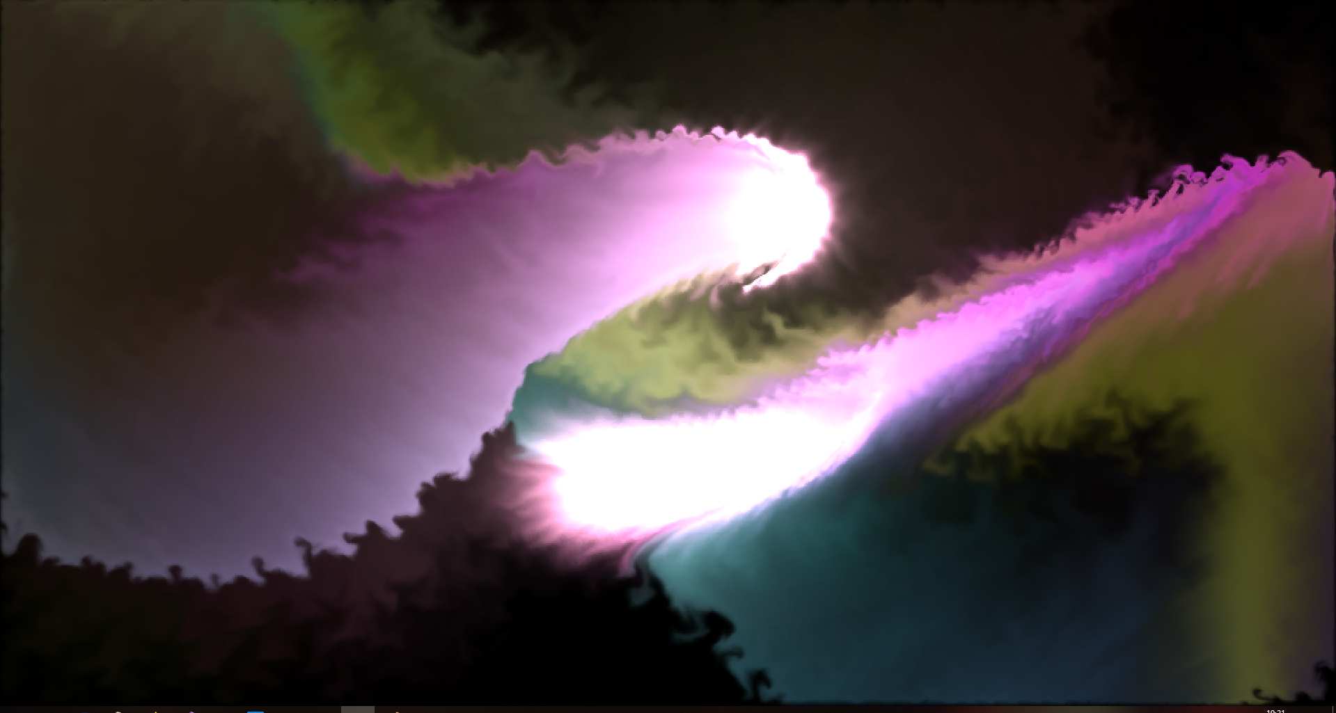
And in the end, a small bonus - a few beautiful screenshots taken in the program:

Direct stream (default settings)

Whirlpool (large radius in applyForce)

Wave (high vorticity + diffusion)
Also, by popular demand, I added a video with the simulation:
All Articles