PDDM - New Model-Based Reinforcement Learning Algorithm with Advanced Scheduler

Reinforcement Learning is divided into two large classes: Model-Free and Model-Based. In the first case, actions are optimized directly by the reward signal, and in the second, the neural network is only a model of reality, and the optimal actions are selected using an external scheduler. Each approach has its own advantages and disadvantages.

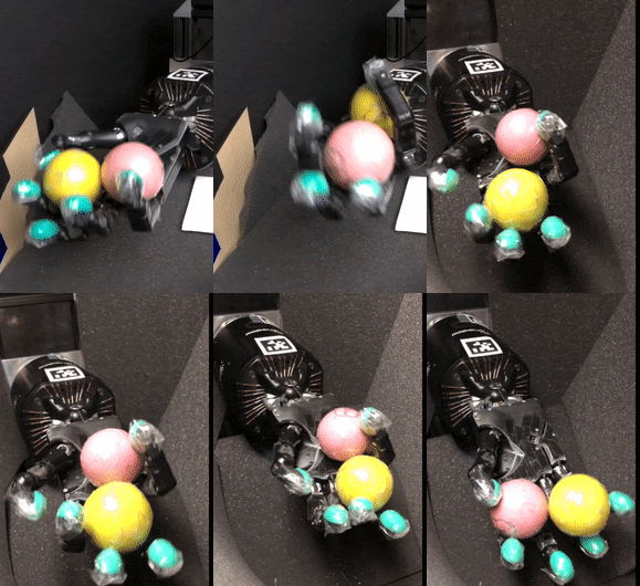
Developers from Berkeley and Google Brain introduced the Model-Based PDDM algorithm with an improved scheduler, which allows you to effectively learn complex movements with a large number of degrees of freedom with a small number of examples. To learn how to rotate balls in a robotic arm with realistic finger joints with 24 degrees of freedom, it took only 4 hours of practice on a real physical robot.

Reinforcement Learning is the training of robots with a reward signal. This is similar to how living beings learn. But the problem is complicated by the fact that it is not known how to change the weights of the neural network so that its proposed actions lead to an increase in rewards. Therefore, in Reinforcement Learning, conventional neural network training methods are not suitable. After all, it is not known what exactly she should give out at her exit, which means it is impossible to find an error between her prediction and the real state of things. To skip this difference back through the layers of the neural network and change the weights between the neurons to minimize this error. This is a classic back-propagation algorithm taught by neural networks.

Therefore, scientists have invented several ways to solve this problem.

Model-free

One of the most effective approaches was the actor-critic model. Let one neural network (actor) at its input receive the state of the state environment, and at the output, issue actions that should lead to an increase in reward rewards. So far, these actions are random and simply depend on the signal flow within the network, since the neural network has not yet been trained. And let the second neural network (critic) also receive the state of the state environment, but also actions from the output of the first network. And at the output, let only the reward reward predicted, which will be received if these actions are applied.

Now watch your hands: we don’t know what optimal actions should be at the output of the first network, leading to an increase in reward. Therefore, using the back propagation algorithm, we cannot train it. But the second neural network can very well predict the exact value of the reward reward (or rather, usually its change), which it will receive if actions are now applied. So let's take the error change gradient from the second network, and apply it to the first! So you can train the first neural network by the classical method of back propagation of error. We simply take the error not from the outputs of the first network, but from the outputs of the second.

As a result, the first neural network learns to issue optimal actions leading to an increase in rewards. Because if the critic critic made a mistake and predicted a smaller reward than turned out to be in reality, then the gradient of this difference will move the actions of the actor actor in the direction so that the critic more accurately predicts the reward. And that means towards more optimal actions (after all, they will lead to the fact that the critic will accurately predict a higher award). A similar principle works in the opposite direction: if the critic overestimates the expected reward, the difference between expectation and reality will lower the actions outputs of the first neural network, which led to this overestimated reward indication of the second network.

As you can see, in this case, the actions are optimized directly by the reward signal. This is the common essence of all Model-Free algorithms in Reinforcement Learning. They are the state-of-the-art at the moment.

Their advantage is that optimal actions are sought by gradient descent, therefore, in the end, the most optimal ones are found. Which means showing the best result. Another advantage is the ability to use small (and therefore faster learnable) neural networks. If out of the whole variety of environmental factors some specific ones are key to solving the problem, then gradient descent is quite capable of identifying them. And use to solve the problem. These two advantages have ensured success with direct Model-Free methods.

But they also have disadvantages. Since actions are taught directly by the reward signal, many training examples are needed. Tens of millions, even for very simple cases. They work poorly on tasks with a large number of degrees of freedom. If the algorithm does not immediately manage to identify key factors among the landscape of high dimension, then it most likely will not learn at all. Also Model-Free methods can exploit vulnerabilities in the system, focusing on non-optimal action (if gradient descent converges on it), ignoring other environmental factors. For even slightly different Model-Free tasks, methods have to be trained completely again.

Model-based

The model-based methods in Reinforcement Learning are fundamentally different from the approach described above. In Model-Based, a neural network only predicts what will happen next. Not offering any action. That is, it is simply a model of reality (hence the "Model" -Based in the name). And not a decision-making system at all.

Model-Based neural networks are fed with the current state of the state environment and which actions we want to perform. And the neural network predicts how the state will change in the future after applying these actions. She can also predict what reward will be as a result of these actions. But this is not necessary, as the reward can usually be calculated from a well-known state. Further, this output state can be fed back to the input of the neural network (along with new proposed actions), and so recursively predict changes in the external environment many steps forward.

Model-based neural networks are very easy to learn. Since they simply predict how the world will change, without making any suggestions what optimal actions should be in order for the reward to increase. Therefore, the Model-Based neural network uses all existing examples for its training, and not just those that lead to an increase or decrease in rewards, as is the case in Model-Free. This is the reason why Model-Based neural networks need much less training examples.

The only drawback is that Model Based neural network should study the real dynamics of the system, and therefore should have sufficient capacity for this. A Model-Free neural network can converge on key factors, ignoring the rest, and therefore be a small simple network (if the task is in principle solved by fewer resources).

Another great advantage, in addition to training on a much smaller number of examples, is that as a universal model of the world, a single Model-Based neural network can be used to solve any number of problems in this world.

The main problem in the Model-Based approach is what actions actions should be applied to the input of neural networks? After all, the neural network itself does not offer any optimal actions.

The easiest way is to drive through such a neural network tens of thousands of random actions and choose those for which the neural network will predict the greatest reward. This is a classic Model-Based Reinforcement Learning. However, with large dimensions and long time chains, the number of possible actions turns out to be too large to sort through them all (or even guess at least a little optimal).

For this reason, Model-Based methods are usually inferior to Model-Free, which by gradient descent directly converge to the most optimal actions.

An improved version applicable to movements in robotics is not to use random actions, but to keep the previous movement, adding randomness to the normal distribution. Since the movements of robots are usually smooth, this reduces the number of busts. But at the same time, an important sharp change can be missed.

The final development option for this approach can be considered the CEM option, which uses not a fixed normal distribution that introduces randomness into the current path of actions, but selects the parameters of the random distribution using cross-entropy. To do this, a population of actions calculations is launched and the best of them are used to refine the spread of parameters in the next generation. Something like an evolutionary algorithm.

PDDM

Such a long introduction was needed in order to explain what is happening in the new proposed PDDM Model-Based reinforcement learning algorithm. After reading an article on the Berkeley AI blog (or an extended version ), and even the original article arxiv.org/abs/1909.11652 , this might not have been obvious.

The PDDM method repeats the idea of ​​CEM when choosing random actions that need to be run through a Model-Based neural network in order to select actions with the highest predictable reward. Only instead of selecting random distribution parameters, as is done in CEM, PDDM uses a temporal correlation between actions and a softer rule for updating random distribution. The formula is given in the original article. This allows you to check a larger number of suitable actions over long time distances, especially if movements require precise coordination. In addition, the authors of the algorithm filter candidates for actions, thereby obtaining a smoother trajectory of movements.

Simply put, the developers simply proposed a better formula for choosing random actions to test in classic Model-Based Reinforcement Learning.

But the result was very good.

In just 4 hours of training on a real robot, a robot with 24 degrees of freedom learned to hold two balls and rotate them in the palms without dropping them. An unattainable result for any modern Model-Free methods with such a small number of examples.

Interestingly, for training, they used a second robot arm with 7 degrees of freedom, which picked up the dropped balls and returned them to the main robot arm:

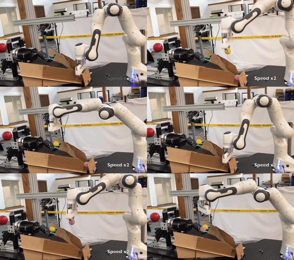
As a result, after 1-2 hours, the roboruk could confidently hold the balls and move them in the palm of her hand, and 4 hours was enough for complete training.

Pay attention to the twitching movements of the fingers. This is a feature of Model-Based approaches. Since the intended actions are chosen randomly, they do not always coincide with the optimal ones. The Model-Free algorithm could potentially converge on truly optimal smooth movements.

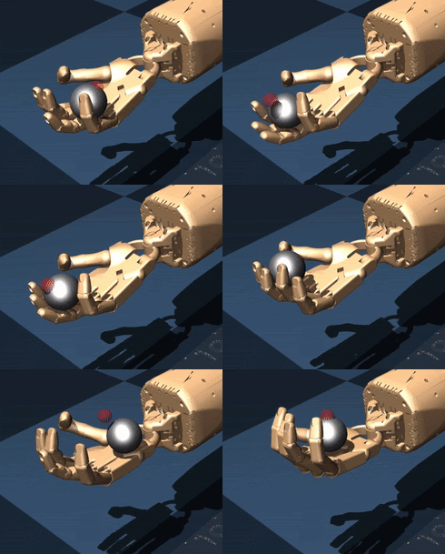
However, the Model-Based approach allows with one trained neural network modeling the world to solve different problems without retraining. There are several examples in the article, for example, you can easily change the direction of rotation of the balls in the hand (in Model-Free, you would have to re-train the neural network for this). Or hold the ball at a specific point in the palm of your hand, following the red dot.

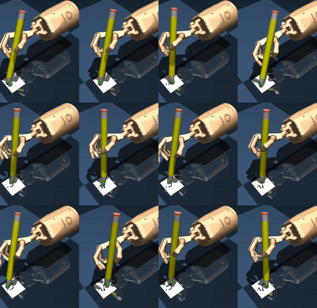
You can also make Roboruk draw arbitrary paths with a pencil, learning which for Model-Free methods is a very difficult task.

Although the proposed algorithm is not a panacea, and is not even an AI algorithm in the full sense of the word (in PDDM, the neural network simply replaces the analytical model, and decisions are made by random search with a tricky rule that reduces the number of enumeration of options), it can be useful in robotics. Since it showed a noticeable improvement in results and is trained on a very small number of examples.