How alpha compositing works
Transparency may not seem like an interesting topic. The GIF format, which allowed some pixels to shine through the background, was published over 30 years ago. Almost every graphic design application released over the past two decades supports the creation of translucent content. These concepts have long ceased to be something new.
In my article I want to show that in fact transparency in digital images is much more interesting than it seems - in what we take for granted, there is an invisible depth and beauty.
Opacity
If you have ever seen through pink glasses, then you could see something similar to what is shown in the figure below. [In the original article, many images are interactive.] Try moving the glasses to see how they affect what is visible through them:

Such glasses work as follows: they miss a lot of red, a decent amount of blue and very little green. The mathematics of these points can be written in a set of three equations. The letter R indicates the result of the operation, and the letter D describes the point we are looking at. RGB indices denote red, green, and blue components:
R R = D R × 1.0
R G = D G × 0.7
R B = D B × 0.9
This colored glass transmits red, green and blue components of the background with different strengths. In other words, the transparency of pink glasses depends on the color of the incident light. In the general case, transparency may vary depending on the wavelength of light , but in this simplified example, we are only interested in how glasses affect the classic RGB components.
Simulating the behavior of ordinary sunglasses is much simpler, they usually just attenuate the incident light by some amount:

These glasses allow only 30% of the light passing through them. Their behavior can be described by the following equations:
R R = D R × 0.3
R G = D G × 0.3
R B = D B × 0.3
All three color components are reduced by the same value - the absorption of incident light is the same. We can say that dark glasses are 30% transparent (opaque) or that they are 70% opaque. The opacity of an object determines how much color it blocks. In computer graphics, we usually deal with a simplified model in which only one value is needed to describe this property. Opacity can vary spatially. like, for example, a column of smoke that is becoming higher and more transparent.
In the real world, objects with an opacity of 100% are simply opaque and they do not transmit light at all. The world of digital images is a little different. There are borderline cases in it, when even solid opaque objects pass a certain amount of light.
Coating
Vector graphics deals with clear and infinitely accurate descriptions of shapes defined with dots. line segments, Bezier curves and other mathematical primitives. When you need to display figures on a computer screen, these impeccable entities have to be rasterized into a bitmap:

Rasterization of a vector shape to a bitmap
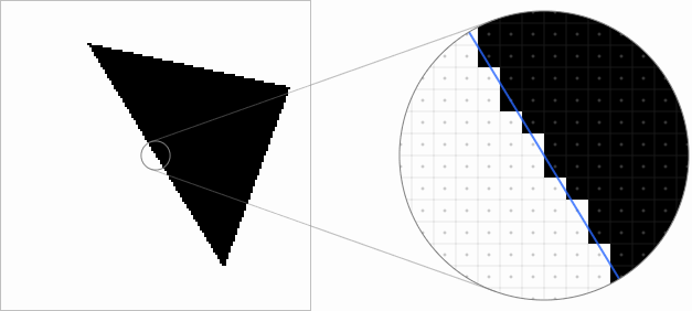
The most primitive way to rasterize is to check where the pixel sample is located inside or outside the vector shape. In the examples below, you can drag the triangle, in an enlarged view, the movements will be more accurate. The blue outline indicates the original vector geometry. As you can see, the ladder at the edges of the triangle looks ugly and flickers a lot when moving the geometry:
The disadvantage of this approach is that we perform only one check for each displayed pixel, and the results are discretized to one of two possible values - inside or outside.
You can sample vector geometry several times per pixel to get a large gradation of steps and decide that some pixels are only partially closed. One possible solution is to use four sampling points to represent five coverage levels: 0, 1 ⁄ 4 , 2 ⁄ 4 , 3 ⁄ 4, and 1:

The quality of the edges of the triangle has improved, but just five possible levels of coverage are often not enough and we can easily achieve a much better result. Although the view of the pixel as a small square in the world of signal processing is viewed with disapproval , in some contexts it is a useful model that allows us to calculate the exact coverage of a pixel by vector geometry. The intersection of a line and a square can always be decomposed into a trapezoid and a rectangle :

A line segment divides a square into a trapezoid and a rectangle
You can easily calculate the area of both parts, and their sum divided by the area of the square determines the percentage of pixel coverage. Thus, the coverage is calculated as an exact number with arbitrary accuracy. In the demo shown below, this method is used to render much better edges that remain smooth even when dragging a triangle:

When it comes to more complex shapes, for example, ellipses or Bezier curves , they are often divided into simple line segments that allow you to calculate the coverage with the required accuracy.
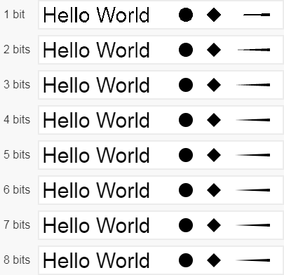
The concept of partial coverage is critical for high-quality rendering of vector graphics and, more importantly, for rendering text. If you take a screenshot of this article and consider it carefully, you will notice that almost all edges of the glyphs cover pixels only partially:

Partial coverage is actively used in text rendering
Having the opacity of the object and covering it with individual pixels, you can combine them into one value.
Alpha
The product of the opacity of an object and its pixel coverage is called alpha :
= ×
An object with an opacity of 60%, covering 30% of the pixel area, has an alpha value of 18% in this pixel. Naturally, when an object is transparent or completely does not cover a pixel, the alpha value in this pixel is 0. After multiplication, the differences between opacity and coating disappear, which in a sense justifies the fact that the concepts of “alpha” and “opacity” are used synonymously.
Alpha is often represented as a fourth channel of a bitmap image. The usual values of red, green and blue are complemented by an alpha value, forming a four RGBA values.
When it comes to storing alpha values in memory, there is a temptation to use just a few bits for this. In the case of covering the pixels of the edges of opaque objects, it seems that 4 or even 3 bits will be quite enough, depending on the pixel density of the screen:
However, opacity also affects the alpha value, so low bit depth can be catastrophic in some cases of smoothly changing transparency. The image below shows a gradient from opaque black to white, which demonstrates that low bit depth leads to very strong color variations:
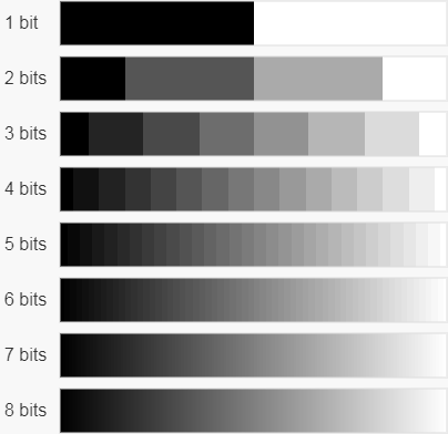
Obviously, the more bits, the better, and most often alpha 8 uses a bit depth of 8 to match the accuracy of the color components, which is why many RGBA buffers occupy 32 bits per pixel. It is also worth noting that, unlike color components, which are often encoded using non-linear transformation, alpha is stored linearly - the encoded value of 0.5 corresponds to an alpha value of 0.5.
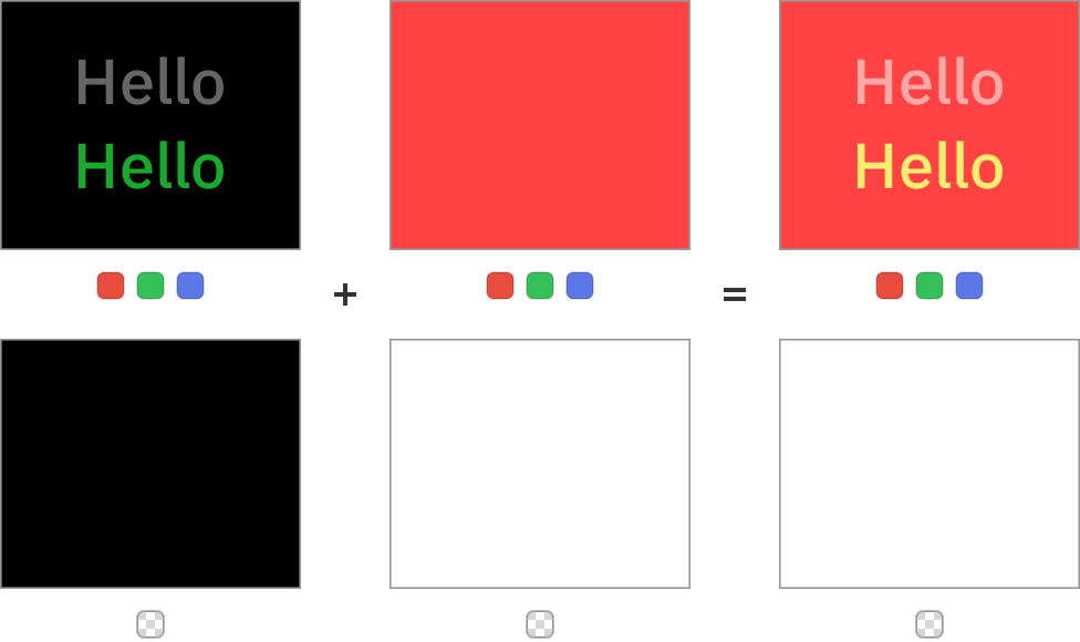
Speaking about alpha, we have completely ignored all other color components, but in addition to blocking the background color, the pixel itself can add a little color. The idea is quite simple - a translucent pink object blocks part of the incoming background lighting and emits or reflects a little pink light:

Notice that it does not behave like stained glass. Glass simply blocks part of the background lighting with different brightness. If you look at a completely black object through pink glass, then its blackness will remain, because the black object does not emit and does not reflect any light. However, the translucent pink object adds its own light. If you place it on top of a black object, the result will be pinkish. A good analogue of this behavior is fine material suspended in the air, such as haze, smoke, fog or some colored powder.
Rendering the alpha channel is a little more difficult - a perfectly transparent object is invisible by definition, so to distinguish between objects, we need to use two tricks. A checkerboard background shows which parts of the image are transparent; This pattern is used in many graphical applications:

Chess pattern shows transparent pieces.
The four small squares below the image tell us that we see the red, green, blue and alpha components of the image. In some cases, it is useful to directly see the alpha channel values, and the easiest way to display them is using shades of gray:

Display RGB and A values on different surfaces
The brighter the shade of gray, the higher the alpha value, that is, pure black corresponds to 0% alpha, and pure white to 100% alpha. Small squares indicate that the RGB and A components of the image are divided into two parts.
The alpha component itself is not particularly useful, but it becomes very important when we talk about compositing.
Simple compositing
Very few 2D rendering effects can be implemented in one operation, and to create a finished result, we use a compositing process that combines different images. For example, a simple “Cancel” button can be created by compositing five separate elements:

Compositing Elements for the Cancel Button
Compositing is often performed in several stages, at each of which two images are combined. The foreground image used in compositing is commonly called source . The background image used in compositing, on which source is superimposed, is usually called destination .
We will start by compositing on an opaque background, because this is a very common case. Everything that you see on the screen is ultimately superimposed by compositing on an opaque destination.
When the alpha value of source is 100%, then source is opaque and should completely cover destination. If the alpha value is 0%, then source is completely transparent and does not affect destination in any way. An alpha value of 25% allows the object to emit 25% of its light and passes 75% of the light from the background, and so on:

Composing purple source with different alpha values to yellow destination
You can already understand what everything is going to - a simple case of alpha compositing on an opaque background - this is just linear interpolation between the destination and source colors. In the graph below, the slider controls the alpha value of the source, and the red, green, and blue graphs display the values of the RGB components. The result of R is just a mix between source S and destination D :
What happens here can be described by the equations shown below. As before, the index denotes the component, that is, S A is the alpha value in source, and D G is the green value in destination:
R R = S R × S A + D R × (1 − S A )
R G = S G × S A + D G × (1 − S A )
R B = S B × S A + D B × (1 − S A )
The equations for the red, green, and blue components have the same appearance, so you can simply use the RGB index and combine them into one line:
R RGB = S RGB × S A + D RGB × (1 − S A )
Moreover, since destination is opaque and already blocks all background light, we know that the alpha value of the result is always 1:
R A = 1
Compositing on an opaque background is simple, but it is quite limited in capabilities. In many cases, a more reliable solution is required.
Intermediate buffers
The image below shows the two-step process of compositing three different layers, labeled A, B, and C. The symbol ⇨ will mean "superimposed by compositing on":

The result of two-stage compositing of three layers
First we overlay B with C by composing, and then overlay A with them to get the finished image. In the following example, we will do things a little differently. First, we will connect the top two layers by compositing, and then overlay the result on the last destination:

The result of two-stage compositing of three layers in a different order
You are probably wondering if such a situation arises in practice, but in fact it is very common. Many non-trivial compositing operations and rendering effects, such as masking and blurring, require passing through an intermediate buffer containing only partial compositing results. This concept has different names: offscreen passes, transparency layers, or side buffers, but usually they are based on the same idea.
What is more important for us is that almost any image with transparency can be perceived as a partial result of some rendering, which will later be superimposed by compositing on the last destination:
Partial compositing of a button into a clipboard
We need to understand how to replace the compositing of translucent images A and B with one image (A⇨B) having the same color and opacity. Let's start by calculating the alpha value of the final buffer.
Combining alpha values
It may not be clear to you how to combine the opacity of two objects, but it’s easier to talk about this task if we talk about transparency instead.
Suppose a certain amount of light passes through the first object, and then through the second object. If the transparency of the first object is 80%, then it will pass 80% of the incident light. Similarly, a second object with 60% transparency will let in 60% of the light passing through it, which gives us 60% × 80% = 48% of the original light. You can experiment with transparency in the original article; do not forget that the sliders control the transparency and not the opacity of objects in the path of light:

Naturally, when either the first or second object is opaque, no light passes through them, even another is completely transparent.
If object D has transparency D T , and object S has transparency S T , then the final general transparency R T of these two objects is equal to their product:
R T = D T × S T
However, transparency is just a unit minus alpha, so substitution gives us the following:
1 - R A = (1 - D A ) × (1 - S A )
This expression can be expanded into:
1 - R A = 1 - D A - S A + D A × S A
And simplify it like this:
R A = D A + S A - D A × S A
It can be reduced to one of two similar types:
R A = S A + D A × (1 - S A )
R A = D A + S A × (1 - D A )
Soon we will see that the second is more often used. It is also interesting to note that the resulting alpha value does not depend on the relative order of the objects - the opacity of the resulting pixels is the same, even if you swap the source and destination. This is very logical. The light passing through two objects should fade out the same way, from whatever side of the star, from the front or from the back.
Color combination
Calculating alpha was not so difficult, so let's try to understand the calculations of RGB components. The source image has the color S RGB , but its opacity S A forces only the product of these two values into account in the finished result:
S RGB × S A
The destination image has the color D RGB , the opacity makes it emit light D RGB × D A , however, part of the light is blocked by the opacity of the image S, so all the influence of destination is equal to:
D RGB × D A × (1 - S A )
The total contribution of light from S and D is equal to their sum:
S RGB × S A + D RGB × D A × (1 - S A )
Similarly, the contribution of the merged layers is equal to their color times their opacity:
R RGB × R A
We want these two values to match:
R RGB × R A = S RGB × S A + D RGB × D A × (1 - S A )
What gives us the final equations:
R A = S A + D A × (1 - S A )
R RGB = (S RGB × S A + D RGB × D A × (1 - S A )) / R A
See how complicated the second equation is! Note that to get the RGB values of the result, we need to divide by the alpha value. However, for the next stage of the compositin, multiplication by the alpha value will again be required, because the result of the current operation will become the new source or destination of the next operation. It is simply ugly.
Let's go back to the almost final form of R RGB for a second:
R RGB × R A = S RGB × S A + D RGB × D A × (1 - S A )
Source, destination and result are multiplied by their alpha components. This makes us understand that the color and alpha of the pixel “like” to be together, so we need to take a step back and rethink the way we store color information.
Premultiplied alpha
Recall that we talked about opacity - if the object is partially opaque, then its contribution to the result will also be partial. The concept of Premultiplied alpha (“pre-multiplication by alpha”) implements this idea. The values of the RGB components, as the name implies, are preliminarily multiplied by the alpha component. Let's start with color without preliminary multiplication:
(1.00, 0.80, 0.30, 0.40)
Preliminary multiplication by alpha gives us the following:
(0.40, 0.32, 0.12, 0.40)
Let's take a look at several pixels at a time. The figure below shows how color information is stored without first multiplying alpha:

RGB and A information in the image without prior multiplication
Note that areas where alpha is 0 can have arbitrary RGB values, as can be seen from the green and blue glitches in the image. In the case of preliminary multiplication by alpha, the color information also stores pixel opacity values:

RGB and A information in a pre-multiplied image
Premultiplied alpha is sometimes called associated alpha, and non-premultiplied alpha is sometimes called straight or unassociated alpha.
When the alpha component of the color is 0, preliminary multiplication resets all other components, regardless of their values:
(0.0, 0.0, 0.0, 0.0)
In the case of premultiplied alpha, there is only one completely transparent color, and this is charming.
The advantages of this processing of color components will gradually become clear to you, but before we return to the compositing example, let's see how premultiplied alpha helps solve some other rendering problems.
Filtration
Gaussian blur is a popular way to create an interesting defocused background or reduce the high frequency of the background part of the contents of some UI elements. As we will see, pre-multiplying alpha is critical to creating the right looking blur.
The image that we will analyze is created by filling the background with 1% opaque blue, over which an opaque red circle is drawn. First, let's look at an example without preliminary multiplication. I separated the RGB channels from the alpha channel to understand what was going on. The arrow indicates the blur operation:

Blur content without preliminary multiplication
The finished result has an ugly blue halo. It happened because the blue background leaked onto the red area during the blur, and only then , during compositing, the alpha weight was added to it.
When the colors are pre-multiplied by alpha, the result is correct:

Blurring pre-multiplied content
Due to pre-multiplication, the blue color of the image is reduced to 1% of its original strength, so its effect on the colors of the blurred circle is extremely small.
Interpolation
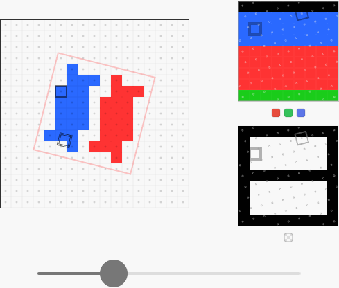
Rendering an image whose pixels fit perfectly with destination is a simple task because we need to perform a trivial one-to-one mapping between samples. A problem arises when there is no simple mapping, for example, due to rotation, scaling, or hyphenation. The figure below shows that the pixels of the rotated image indicated by the red outline no longer match the destination:

Relative image orientation and destination pixels before and after rotation
There are many ways to select a color from the image to be written to the destination pixel, and the simplest of them is the so-called nearest-neighbor interpolation, in which as the final pixel, the closest sample in the texture is simply selected.
In the demo shown below, the red outline shows the position of the image in destination. On the right are sample positions from the image point of view . By dragging the slider (in the original article), you can rotate the quadrangle and observe how the samples select colors from the bitmap. I highlighted one pixel in source and destination, so that their relationship is more clear:
This solution is quite functional and the pixels have a holistic color, but the quality is unacceptable. It would be better to use bilinear interpolation , which calculates the weighted average of the four nearest pixels of the sampled image:
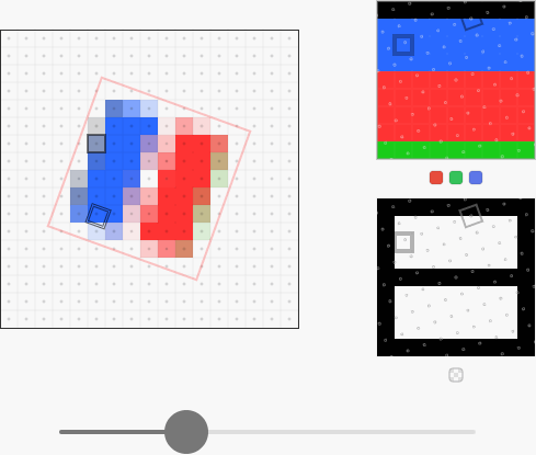
This works better, but the edges around the rectangles do not look right, the contents of the pixels merge without multiplication, because alpha is "applied" after interpolation. Sometimes the recommended solution to merging the color of the right content, which is shown in the amazing article by Adrian Correger [ translation on Habré], is far from ideal - not a single color in the gap between the red and blue rectangles will look right.
Let’s see how everything will look in the image with premultiplied alpha and compositing with an advanced formula, which we will soon derive:
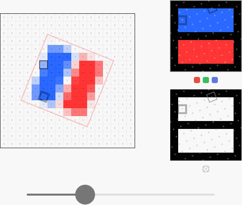
Just perfect - we got rid of all the fusions of colors and the teeth are nowhere to be seen .
Ultimately, the problems associated with blurring and interpolation are closely related. Any operation that requires any combination of translucent colors, without first multiplying the colors by alpha, is likely to give incorrect results.
Proper compositing
Let's get back to compositing. We settled on an almost derived equation:
R RGB × R A = S RGB × S A + D RGB × D A × (1 - S A )
If you imagine colors using premultiplied alpha, then all these uncomfortable multiplications will disappear, because alpha will already be part of the color values. Then we get the following:
R RGB = S RGB + D RGB × (1 - S A )
Let's look at the alpha equation:
R A = S A + D A × (1 - S A )
The coefficients for the red, green, blue and alpha channels are the same, so we can express the whole expression with one equation and just remember that each component undergoes the same operation:
R = S + D × (1 - S A )
See how premultiplied alpha made things easy. When we analyze the components of an equation, they are all in place. The operation masks part of the background light and adds a new light:
R = S + D × (1 - S A )
This mixing operation is called source-over, sover, or simply normal, and it is without a doubt the most common compositing mode. Almost everything you see on my website is mixed in this mode.
Associativity
An important source-over property performed on pre-alpha-multiplied colors is the associativity of this operation. Thanks to him, in the complex mixing equation, we can place the brackets completely arbitrarily. All of the compositions shown below are equivalent:
R = (((A⇨B) ⇨C) ⇨D) ⇨E
R = (A⇨B) ⇨ (C⇨ (D⇨E))
R = A⇨ (B⇨ (C⇨ (D⇨E)) )
The proof of this is simple enough, but I will not burden you with algebraic manipulations. In practice, this means that we can partially render complex drawings without fear that the final composition will look wrong.
In the vast majority of cases, alpha is used only for compositing using source-over, but its advantages do not end there. Alpha values can also be used for other useful rendering operations.
Porter-Duff Compositing
In July 1984, Thomas Porter and Tom Duff published the original article, “Compositing Digital Images” . The authors not only first introduced the concept of premultiplied alpha and derived the source-over compositing equation, but also presented a whole family of alpha-compositing operations, many of which are little known, although very useful. New functions are also called operators , because, like adding or multiplying, they perform actions on input values to create an output value.
Over
In further examples, we will use interactive demos showing the operations of various blending modes. The destination image will be the black “club” symbol, and the source image will be the red “worms” symbol. You can drag the heart over the image and observe how the overlapping shapes behave with different compositing operators. Pay attention to the small minimap in the corner. Some blending modes are very destructive and easy to get confused about. The minimap always shows the result of simple source-over compositing, which simplifies understanding:

R = S + D × (1 - S A )
R = S × (1 - D A ) + D
If you switch to destination-over, then you will immediately realize that it simply “flips” source-over - destination and source are interchanged in the equation and the result is equivalent to what we will consider destination as the source image. Although it seems superfluous, the destination-over operator is extremely useful because it allows you to compose objects that are under existing content.
Out
The source-out and destination-out statements are great for punching holes in source or destination:

R = S × (1 - D A )
R = D × (1 - S A )
Of these two operators, Destination-out is more convenient because it uses the alpha channel to punch holes in the destination form.
In
The source-in and destination-in operators are essentially masking operators:

R = S × D A
R = D × S A
They make it quite easy to create complex intersections of non-trivial geometry without resolving the relatively difficult to compute intersections of vector contours.
Atop
The operators
source-atop
and
destination-atop
allow you to overlay new content on existing ones, while masking it along the destination path:

R = S × D A + D × (1 - S A )
R = S × (1 - D A ) + D × S A
Xor
The exclusive OR operator (
xor
) saves either source or destination, and their matching areas disappear:

R = S × (1 - D A ) + D × (1 - S A )
Source, Destination, Clear
The last three classic compositing modes are pretty boring.
Source
, also called
copy
, just takes the color source. Similarly, it
destination
ignores the color source and simply returns
destination
. The operator
clear
just clears everything:
R = S
R = D
R = 0
The applicability of these modes is limited. Using
clear
it, you can flush a filled buffer, but this operation can be optimized by simply filling the memory with zeros. In addition, in some cases it
source
can be more economical in calculations, because it does not require any mixing, but simply replaces the contents of the buffer with the source information.
Porter Duff in action
Having dealt with individual operators, let's see how you can combine them. In the example below, we will draw a marine logo without using masking or complex geometric shapes. The blue outlines show the simple geometry being created. You can move through the steps by clicking on the right side of the image, and go back by clicking on the left:
Of course, we are by no means obliged to abandon masks and trimming contours, but we often forget about a tool like Porter-Duff compositing modes, although it is much easier to create some visual effects with their help.
Operators
If you look closely at the Porter-Duff operators, you will notice that they all have the same form. Source is always multiplied by a certain coefficient F S and added to destination multiplied by a coefficient F D :
R = S × F S + D × F D
F S can take the values 0, 1, D A + 1 - D A , and F D may be equal to 0, 1, S A or 1 - S A . It makes no sense to multiply source or destination by their own alpha, because they are already pre-multiplied, and we just get a fancy, but not very useful quadratic alpha effect. All operators can be represented in the form of a table:
| 0 | one | D A | 1 - D A | |
| 0 | clear | source | source-in | source-out |
| one | destination | destination-over | ||
| S A | destination-in | destination-atop | ||
| 1 - S A | destination-out | source-over | source-atop | xor |
Pay attention to the symmetry of the operators on the diagonal. The four central elements in the table are missing and it happened because they are different from the rest.
Additive lighting
In their article, Porter and Duff presented another operator in which both F S and F D are equal to 1. It is known by its names
plus
,
lighter
and
plus-lighter
:
R = S + D
This operation essentially adds lighting source to destination:

Additive lighting implemented with the operator
plus
Green and red correctly form yellow, while green and blue form cyan. Black is the absence of an operation; it does not change color values in any way, because adding zero to a number does not change anything.
The three remaining operators were not given names because they are not particularly useful. They are just a combination of masking and blending.
It is also worth noting that premultiplied alpha allows us to use the operator in an
source-over
unexpected way. Let's take a look at the equation again:
R = S + D × (1 - S A )
If we manage to make the alpha value in source equal to zero, then if there are non-zero values in the RGB channels, we can achieve additive lighting without using the operator
plus
:
Additive lighting implemented with the operator
source-over
Note that you need to be careful here - the values are no longer multiplied by alpha correctly. In some programs, there may be an optimization that completely avoids mixing colors with zero alpha, while other programs can reverse pre-multiply by alpha values, perform some color operations, and then pre-multiply again by alpha, which completely destroys the color channels. It can also be difficult to export resources in this format, so if you do not have the ability to fully control the rendering pipeline, then you should stick with the operator
plus
.
All the elements we are discussing have so far been well combined. Now, let's take off our pink glasses and discuss some issues that need to be considered when working with alpha compositing.
Group opacity
Let's take a look at this simple pill drawing made up of just six primitives:
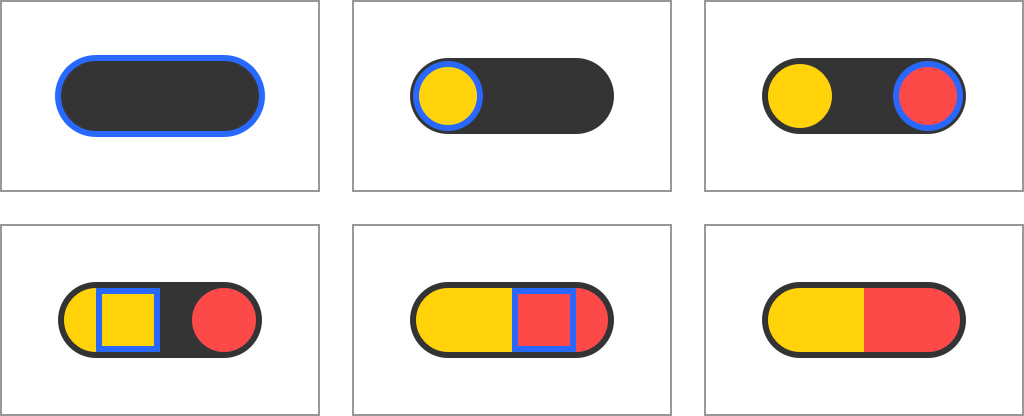
Draw a pill using simple shapes
If we were asked to render a pill with an opacity of 50%, we might be tempted to simply split the opacity in half of each draw operation, but this would turn out to be an erroneous decision:

Unexpected result of rendering a pill with half opacity.
To achieve the correct result, we cannot just distribute the opacity of an object over each of its individual components. We need to first create an object, render it into a bitmap, and only then change the opacity of the bitmap, and finally perform compositing:
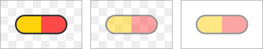
The expected result of rendering a pill with half opacity
This is another case that demonstrates the usefulness of the concept of rendering into a side buffer.
Compositing Coverage
Converting a geometric cover to a single alpha value has uncomfortable consequences. Consider the case when two ideally matching edges of vector geometry figures, shown in the figure below with orange and blue contours, are rendered into a bitmap. In an ideal world, the results should look something like this, because each pixel is completely closed:

An ideal rendering result with the correct coverage.
However, if we first render the orange geometry and then the blue, then in the final image a little white background will still leak into the border pixels:

The result of two-stage compositing
As soon as the coating is saved in the alpha channel, all its geometric information is lost, and we can’t restore it in any way. The blue geometry simply mixes with some of the contents of the buffer, but does not know that the geometry represented by reddish pixels must match it. This problem is especially noticeable when geometries are precisely superimposed on each other. In the image below, a white circle is drawn on top of a black one. Dark edges are noticeable, although both circles have exactly the same radius and position:

A white circle drawn on top of a black circle
One way to fix this problem is to not calculate the partial coverage of the pixels, and use significantly larger buffers. By rasterizing vector geometry with a simple in / out coating, and then reducing the scale of the result to the size of the original image, you can achieve the expected result.
However, for an ideal comparison of the rendering quality of the edges of the 8-bit alpha channel, the buffers should be 256 times larger in both directions, that is, the number of pixels should increase by 2 16time. As we saw above, with a decrease in bit depth for coverage values, satisfactory results can still be obtained, therefore, in practice, a smaller scale can be used.
It is also worth noting that such problems can often be relatively easily avoided without the use of huge bitmaps. For example, instead of drawing two superimposed circles, you can simply draw two squares on top of each other, and then mask the result to form a circle.
Linear values
If you have refreshed your knowledge of color spaces , you can remember that most of them encode color values non-linearly, and preliminary linearization is necessary to perform the correct mathematical operations. When this stage is completed, the result of compositing is as follows; pay attention to the beautiful yellowish shade of the parts superimposed on each other:
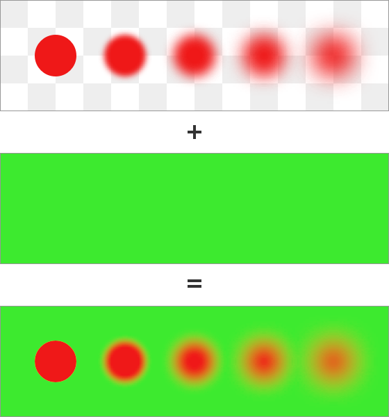
Fuzzy red circles superimposed by compositing on a green background using linear values.
However, in most cases, compositing is not so. The standard way for the web and most graphics software is to directly mix non-linear values:
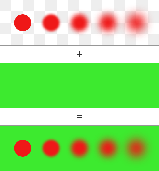
Fuzzy red circles superimposed by a composer on a green background using non-linear values
Note that the areas where the red on green overlays are much darker. They are far from ideal, but in some cases, improper operations are deeply rooted in understanding how we perceive color. For example, 50% opaque gray from the sRGB space looks exactly like pure black with 50% opacity mixed with a white background:

Compositing two colors on a white background without linearization
In the figure below, the sRGB colors of the source and destination images are linearized and then converted back to non-linear encoding for display. Here's how these colors should actually look:

Composition of two colors on a white background with linearization.
We have a discrepancy that does not meet our expectations. The only way to obtain visual uniformity using this method is to select all colors using linear values, but this is very different from what everyone is used to. 50% gray with linear values looks like gray on 73.5% of the sRGB space.
In addition, you need to be especially careful when working with premultiplied alpha. Pre-multiplication must be performed with linear values, i.e. before coding to non-linear. Thanks to this, the linearization step will correctly end with the correct linear values previously multiplied by alpha.
Premultiplied Alpha and Bit Depth
Despite its great utility for compositing, filtering and interpolation, premultiplied alpha is not a “silver bullet” and has its drawbacks. The most serious of them is the reduction in the bit depth of the colors that you can imagine. Imagine an 8-bit encoding of a value of 150, which is pre-multiplied by alpha 20%. After preliminary multiplication by alpha, we get
round (150 × 0.2) = 30
If we repeat the same procedure with a value of 151, we get:
round (151 × 0.2) = 30
The encoded value will be the same, despite the difference in the initial values. In fact, after multiplying by alpha, the values of 148, 149, 150, 151, and 152 are encoded into 30, and the original difference between these five unique colors is lost:

Pre-multiplication by alpha of 20% reduces the various 8-bit values to one.
Naturally, the smaller the alpha, the more destructive is its effect. Of the possible range of 256 4 (approximately 4.3 billion) different combinations of 8-bit RGBA values, after preliminary multiplication by alpha, only 25.2% retain a unique representation; in fact, we lose almost 2 bits from the 32-bit range.
To convert colors between different color spaces, sometimes it is necessary to reverse the preliminary multiplication, that is, divide the values into the alpha component to get the original color brightness. This step is required because, as mentioned above, encoding is performed non-linearly. The existence of pre-multiplication reduces the accuracy of color representation and conversions between color spaces may not be ideal.
In practice, reducing bit depth is rarely important, especially in compositing. The lower the alpha value, the less visible the color, and the less impact it has on compositing. Ultimately, if you strive for pedantically accurate operations on colors, you will not use their 8-bit representation - for this purpose, formats are much better suitedfloating point .
Additional reading
The concept of the alpha channel was created by Pixar co-founders Elvy Smith and Ed Catmell . Smith's article “Alpha and the History of Digital Compositing” describes the history of the invention and the sources of the name “alpha”, as well as how these concepts evolved and gradually replaced the concept of masks in film production .
To understand the meaning of alpha, I highly recommend that you read Andrew Glassner's “Interpreting Alpha” . This article provides a rigorous but very accessible mathematical derivation of alpha as a measure of the interaction between opacity and coverage.
A detailed discussion of premultiplied alpha can be explored in“GPUs prefer premultiplication” by Eric Haines. The article not only provides an excellent overview of the problems caused by the lack of preliminary multiplication, especially in 3D rendering, but also provides links to many other articles on this topic.
Finally
Initially, this article was conceived as an explanation of the Porter-Duff compositing operators, but all the other concepts related to alpha compositing turned out to be so interesting that I could not miss them.
What I like most about alpha is that it's just an extra number that accompanies the RGB components, but at the same time it creates many unique rendering capabilities. Alpha literally created a new change of opportunity in the boring old world of compositing and 2D rendering.
The next time you see the smooth edges of vector shapes or notice a dark overlay that obscures some parts of the user interface, think of a small but powerful component that made it all possible.
All Articles