Hello!



Here we describe the work of a certain field and then make a couple of beautiful features (everything is VERY simple here).







What will happen in this article.



General case:

1. We describe the base, namely, work with vectors (a bicycle for those who do not have numpy on hand)
2. We describe the material point and field of interaction

Special case (based on general):

1. Let's make a visualization of the vector field of the electromagnetic field strength (first and third pictures)
   
   
2. Let's visualize the movement of particles in an electromagnetic field
   
   

Meet me under the cut!

Theoretical Programming

Vector

The basis of all the foundations is the vector (especially in our case). Therefore, it is with the description of the vector that we will begin. What we need? Arithmetic operations on a vector, distance, module, and a couple of technical things. The vector we will inherit from list. This is how its initialization looks:

class Vector(list): def __init__(self, *el): for e in el: self.append(e)
      
      

        
        
        
      

    
        
        
        
      
      

        
        
        
      

    
     

That is, now we can create a vector with

 v = Vector(1, 2, 3)
      
      

        
        
        
      

    
        
        
        
      
      

        
        
        
      

    
     

Let's set the arithmetic operation addition:

 class Vector(list): ... def __add__(self, other): if type(other) is Vector: assert len(self) == len(other), "Error 0" r = Vector() for i in range(len(self)): r.append(self[i] + other[i]) return r else: other = Vector.emptyvec(lens=len(self), n=other) return self + other
      
      

        
        
        
      

    
        
        
        
      
      

        
        
        
      

    
     

Fine:

 v1 = Vector(1, 2, 3) v2 = Vector(2, 57, 23.2) v1 + v2 >>> [3, 59, 26.2]
      
      

        
        
        
      

    
        
        
        
      
      

        
        
        
      

    
     

We similarly define all arithmetic operations (the full code of the vector will be lower). Now you need a distance function. I could make a rustic dist (v1, v2) - but this is not beautiful, so redefine the% operator:

 class Vector(list): ... def __mod__(self, other): return sum((self - other) ** 2) ** 0.5
      
      

        
        
        
      

    
        
        
        
      
      

        
        
        
      

    
     

Fine:

 v1 = Vector(1, 2, 3) v2 = Vector(2, 57, 23.2) v1 % v2 >>> 58.60068258988115
      
      

        
        
        
      

    
        
        
        
      
      

        
        
        
      

    
     

We also need a couple of methods for faster vector generation and beautiful output. There is nothing tricky here, so here is the entire code of the Vector class:

Material point

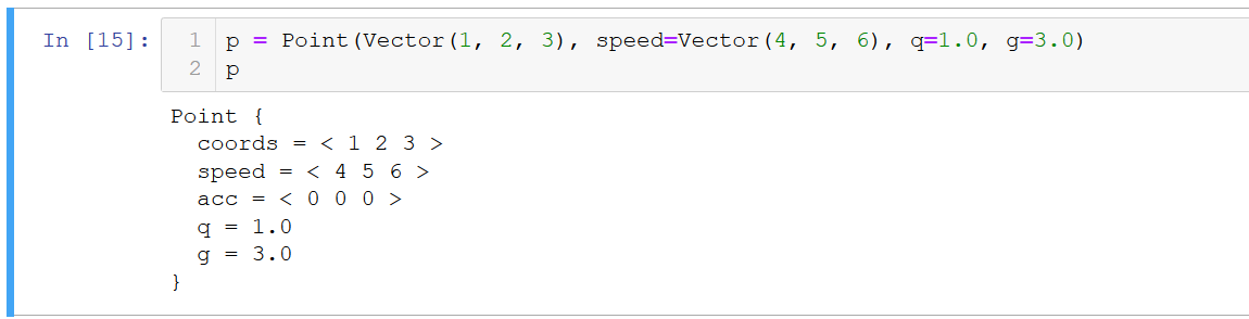
Here, in theory, everything is simple - the point has coordinates, speed and acceleration (for simplicity). In addition, she has a mass and a set of custom parameters (for example, for an electromagnetic field, a charge does not hurt us, but no one bothers you to set at least a spin).



Initialization will be as follows:

 class Point: def __init__(self, coords, mass=1.0, q=1.0 speed=None, **properties): self.coords = coords if speed is None: self.speed = Vector(*[0 for i in range(len(coords))]) else: self.speed = speed self.acc = Vector(*[0 for i in range(len(coords))]) self.mass = mass self.__params__ = ["coords", "speed", "acc", "q"] + list(properties.keys()) self.q = q for prop in properties: setattr(self, prop, properties[prop])
      
      

        
        
        
      

    
        
        
        
      
      

        
        
        
      

    
     

And to move, immobilize and accelerate our point, we will write the following methods:

 class Point: ... def move(self, dt): self.coords = self.coords + self.speed * dt def accelerate(self, dt): self.speed = self.speed + self.acc * dt def accinc(self, force): #        self.acc = self.acc + force / self.mass def clean_acc(self): self.acc = self.acc * 0
      
      

        
        
        
      

    
        
        
        
      
      

        
        
        
      

    
     

Well done, the point itself is done.

Interaction field

We call the field of interaction an object that includes the set of all material points and exerts force on them. We will consider a special case of our wonderful universe, so we will have one custom interaction (of course, this is easy to expand). Declare the constructor and add a point:

 class InteractionField: def __init__(self, F): # F -   , F(p1, p2, r), p1, p2 - , r -    self.points = [] self.F = F def append(self, *args, **kwargs): self.points.append(Point(*args, **kwargs))
      
      

        
        
        
      

    
        
        
        
      
      

        
        
        
      

    
     

Now the fun part is to declare a function that returns “tension” at that point. Although this concept refers to electromagnetic interaction, in our case it is some abstract vector along which we will move the point. In this case, we will have the property of the point q, in the particular case - the charge of the point (in general - whatever we want, even the vector). So what is tension at point C? Something like this:

$$

$$\ vec E (\ vec C) = \ sum {\ vec F_i (\ vec C)}$$

That is the tension at the point $$$\ vec C$ equal to the sum of the forces of all material points acting on some unit point.

 class InteractionField: ... def intensity(self, coord): proj = Vector(*[0 for i in range(coord.dim())]) single_point = Point(Vector(), mass=1.0, q=1.0) #       (   ,       F,      ) for p in self.points: if coord % p.coords < 10 ** (-10): #      ,        ,   ,     (  ) continue d = p.coords % coord fmod = self.F(single_point, p, d) * (-1) #    -  proj = proj + (coord - p.coords) / d * fmod #  return proj
      
      

        
        
        
      

    
        
        
        
      
      

        
        
        
      

    
     

At this point, you can already draw a vector field, but we will do it at the end. Now let's take a step in our interaction

 class InteractionField: ... def step(self, dt): self.clean_acc() for p in self.points: p.accinc(self.intensity(p.coords) * pq) p.accelerate(dt) p.move(dt)
      
      

        
        
        
      

    
        
        
        
      
      

        
        
        
      

    
     

Everything is simple here. For each point, we determine the tension in these coordinates and then determine the final force on the ETU material point:

$$

$$\ vec F = \ vec E * q$$

Define the missing functions.

A special case. Particle movement and vector field visualization

So we got to the most interesting. Let's start with ...

Modeling the motion of particles in an electromagnetic field

 u = InteractionField(lambda p1, p2, r: 300000 * -p1.q * p2.q / (r ** 2 + 0.1)) for i in range(3): u.append(Vector.randvec(2) * 10, q=random.random() - 0.5)
      
      

        
        
        
      

    
        
        
        
      
      

        
        
        
      

    
     

In fact, the coefficient k should be equal to some sort of billions (9 * 10 ^ (- 9)), but since it will be quenched by the time t -> 0, I immediately decided to make both of them adequate numbers. Therefore, in our physics k = 300'000. And with everything else, I think it’s clear.





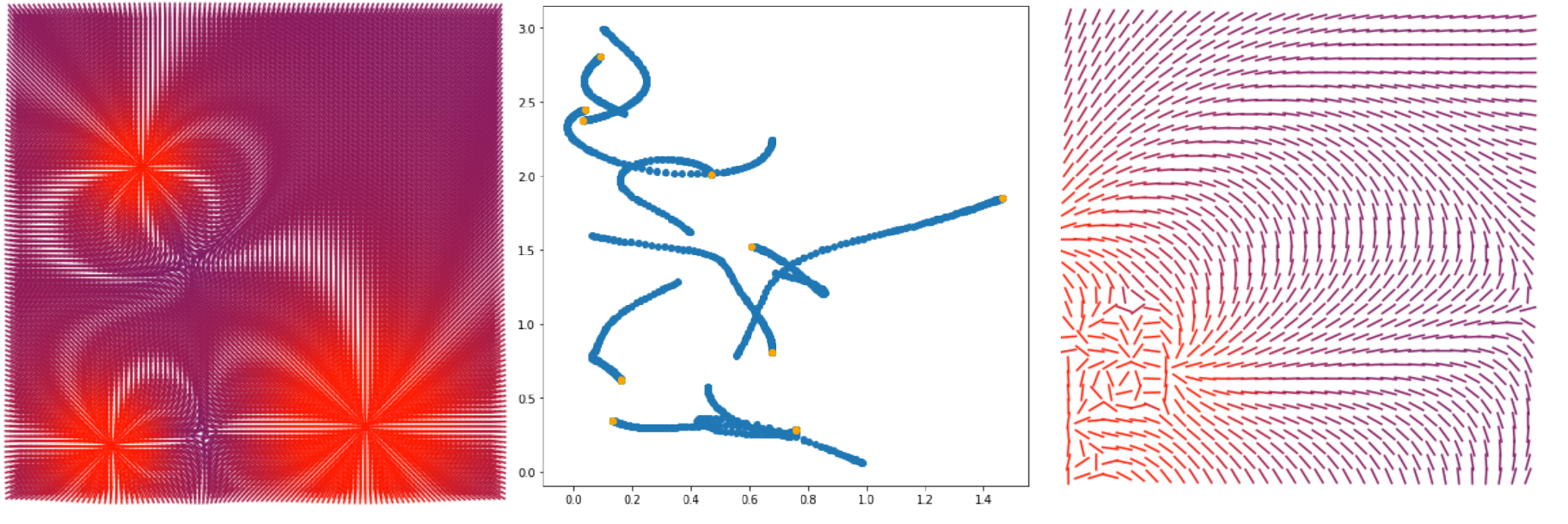
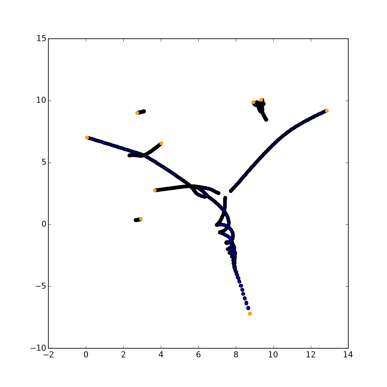
Next, we add ten points (2-dimensional space) with coordinates from 0 to 10 along each axis. Also, we give each point a charge from -0.25 to 0.25. Now make a loop and draw points according to their coordinate (and traces):

 X, Y = [], [] for i in range(130): u.step(0.0006) xd, yd = zip(*u.gather_coords()) X.extend(xd) Y.extend(yd) plt.figure(figsize=[8, 8]) plt.scatter(X, Y) plt.scatter(*zip(*u.gather_coords()), color="orange") plt.show()
      
      

        
        
        
      

    
        
        
        
      
      

        
        
        
      

    
     

What should have happened:







In fact, the pattern there will be completely random, because the trajectory of each point is unpredictable at the moment of the development of mechanics.

Vector field visualization

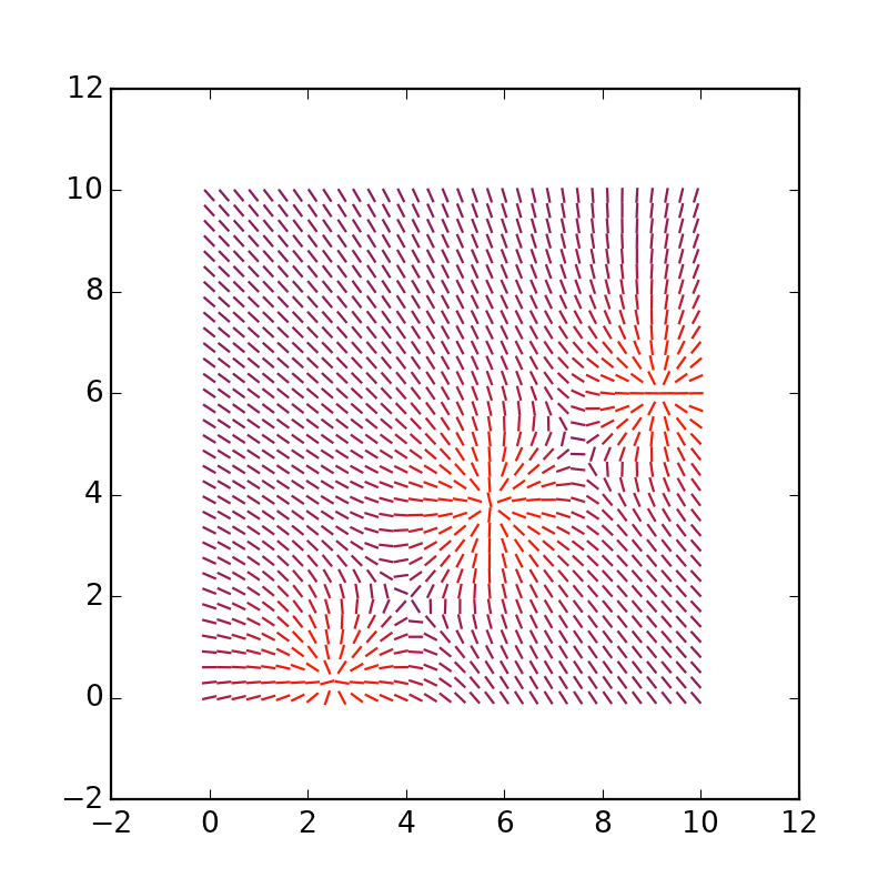
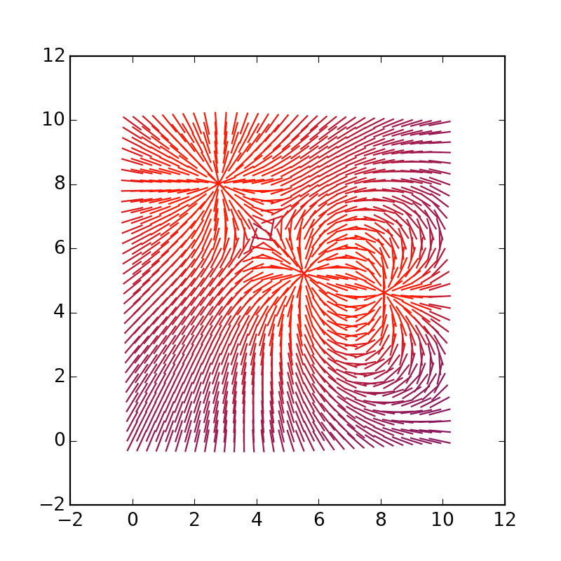
Everything is simple here. We need to go through the coordinates with some step and draw a vector in each of them in the right direction.

 fig = plt.figure(figsize=[5, 5]) res = [] STEP = 0.3 for x in np.arange(0, 10, STEP): for y in np.arange(0, 10, STEP): inten = u.intensity(Vector(x, y)) F = inten.mod() inten /= inten.mod() * 4 #     res.append(([x - inten[0] / 2, x + inten[0] / 2], [y - inten[1] / 2, y + inten[1] / 2], F)) for r in res: plt.plot(r[0], r[1], color=(sigm(r[2]), 0.1, 0.8 * (1 - sigm(r[2])))) #        plt.show()
      
      

        
        
        
      

    
        
        
        
      
      

        
        
        
      

    
     

Approximately this conclusion should have been obtained.







You can lengthen the vectors themselves, replace * 4 with * 1.5:

We play with dimensionality and modeling

Create a five-dimensional space with 200 points and an interaction that is not dependent on the square of the distance, but on the 4th degree.

 u = InteractionField(lambda p1, p2, r: 300000 * -p1.q * p2.q / (r ** 4 + 0.1)) for i in range(200): u.append(Vector.randvec(5) * 10, q=random.random() - 0.5)
      
      

        
        
        
      

    
        
        
        
      
      

        
        
        
      

    
     

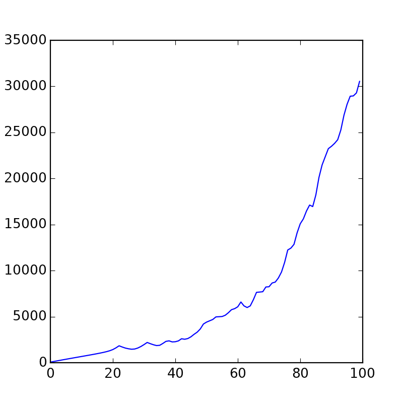
Now all coordinates, speeds, etc. are defined in five dimensions. Now let's model something:

 velmod = 0 velocities = [] for i in range(100): u.step(0.0005) velmod = sum([p.speed.mod() for p in u.points]) #       velocities.append(velmod) plt.plot(velocities) plt.show()
      
      

        
        
        
      

    
        
        
        
      
      

        
        
        
      

    
     

This is a graph of the sum of all speeds at any given time. As you can see, over time they are slowly accelerating.



Well, that was a short instruction on how to make such a simple thing. But what happens if you play with flowers:







The next article will probably be about more complex modeling, and maybe the fluids and Navier-Stokes equations.

UPD: The article was written by my colleague here



Thanks to MomoDev for helping me render the video.