Clustering is an important part of the machine learning pipeline for solving scientific and business problems. It helps to identify sets of closely related (a certain measure of distance) points in the data cloud that could be difficult to determine by other means.



However, the clustering process for the most part relates to the field of machine learning without a teacher , which is characterized by a number of difficulties. There are no answers or tips on how to optimize the process or evaluate the success of the training. This is uncharted territory.



Therefore, it is not surprising that the popular method of clustering by the k-average method does not completely answer our question: “How do we first find out the number of clusters?” This question is extremely important because clustering often precedes the further processing of individual clusters, and from estimating their number depend on the amount of computing resources.



Worst consequences may arise in the field of business analysis. Here, clustering is used for market segmentation, and it is possible that marketing staff will be allocated in accordance with the number of clusters. Therefore, an erroneous estimate of this amount can lead to an non-optimal allocation of valuable resources.

Elbow method

When clustering using the k-means method, the number of clusters is most often estimated using the “elbow method” . It implies multiple cyclic execution of the algorithm with an increase in the number of selectable clusters, as well as subsequent postponement of the clustering score on the graph, calculated as a function of the number of clusters.



What is this score, or metric, which is delayed on the chart? Why is it called the elbow method?



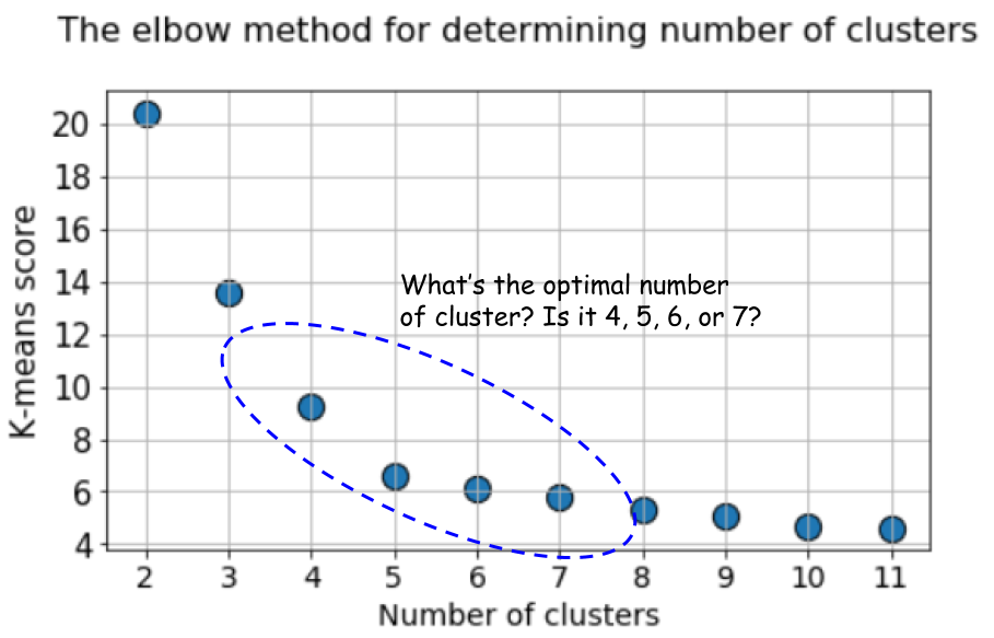
A typical graph looks like this:







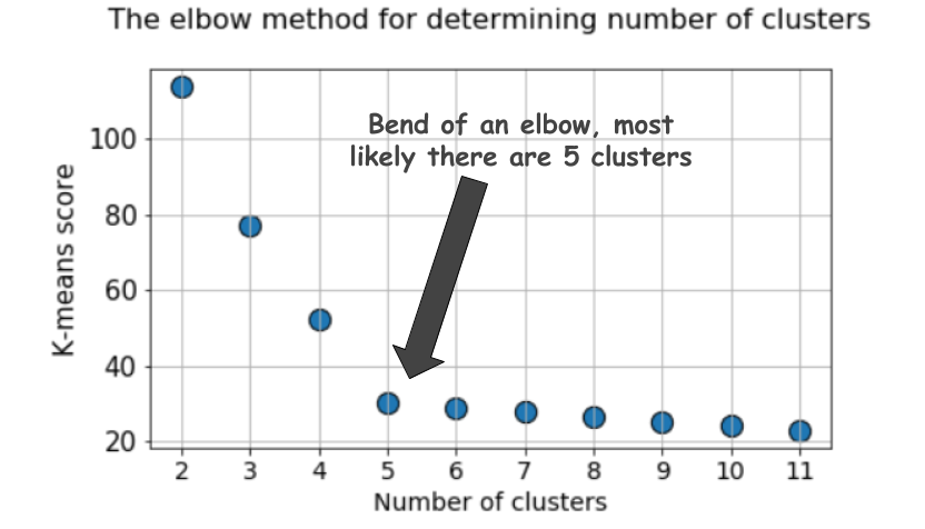
The score, as a rule, is a measure of the input data for the objective function of k-means, that is, some form of the ratio of the intracluster distance to the intercluster distance.



For example, this scoring method is immediately available in the k-means scoring tool in Scikit-learn.



But take another look at this graph. It feels something strange. What is the optimal number of clusters we have, 4, 5 or 6?



It’s not clear, is it?

Silhouette is a better metric

The silhouette coefficient is calculated using the average intracluster distance (a) and the average distance to the nearest cluster (b) for each sample. The silhouette is calculated as (b - a) / max(a, b)



. Let me explain: b



is the distance between a



and the nearest cluster, into which a



does not belong. You can calculate the average silhouette value for all samples and use it as a metric to estimate the number of clusters.



Here is a video explaining this idea:





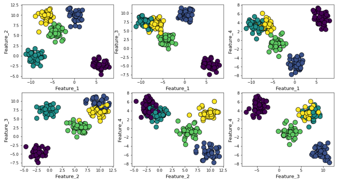
Suppose we generated random data using the make_blob function from Scikit-learn. The data are located in four dimensions and around five cluster centers. The essence of the problem is that the data is generated around five cluster centers. However, the k-means algorithm does not know about this.



Clusters can be displayed on the chart as follows (pairwise signs):







Then we run the k-means algorithm with values ​​from k = 2 to k = 12, and then we calculate the default metric to k-means and the average silhouette value for each run, with the results displayed in two adjacent graphs.







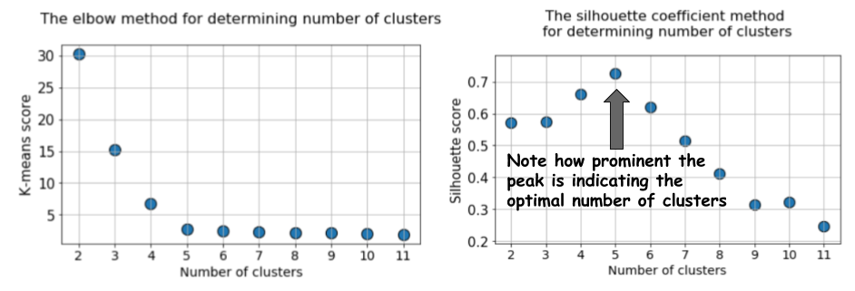
The difference is obvious. The average value of the silhouette increases to k = 5, and then decreases sharply for higher values ​​of k . That is, we get a pronounced peak at k = 5, this is the number of clusters generated in the original dataset.

The silhouette graph has a peak character, in contrast to the softly curved graph when using the elbow method. It is easier to visualize and justify.

If you increase the Gaussian noise during data generation, then the clusters will overlap more strongly.







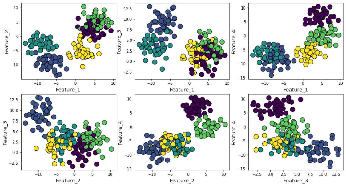
In this case, calculating the default k-means using the elbow method gives an even more uncertain result. Below is a graph of the elbow method, at which it is difficult to choose a suitable point at which the line actually bends. Is it 4, 5, 6 or 7?







At the same time, the silhouette graph still shows a peak in the region of 4 or 5 cluster centers, which greatly facilitates our lives.



If you look at overlapping clusters, you will see that, despite the fact that we generated data around 5 centers, only 4 clusters can be structurally distinguished due to high dispersion. The silhouette easily reveals this behavior and shows the optimal number of clusters between 4 and 5.

BIC score with normal distribution mix model

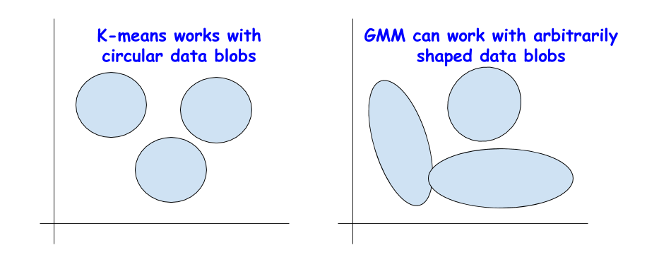
There are other great metrics to determine the true number of clusters, such as the Bayesian Information Criterion (BIC). But they can be used only if we need to switch from the k-means method to a more generalized version - a mixture of normal distributions (Gaussian Mixture Model (GMM)).



GMM views the data cloud as a superposition of numerous datasets with a normal distribution, with separate mean values ​​and variances. And then GMM applies the expectations maximization algorithm to determine these averages and variances.

BIC for regularization

You may already have encountered BIC in statistical analysis or when using linear regression. BIC and AIC (Akaike Information Criterion) are used in linear regression as regularization techniques for the process of selecting variables.



A similar idea applies to BIC. Theoretically, extremely complex clusters can be modeled as superpositions of a large number of datasets with a normal distribution. To solve this problem, you can apply an unlimited number of such distributions.

But this is similar to increasing the complexity of the model in linear regression, when a large number of properties can be used to match data of any complexity, only to lose the possibility of generalization, since an overly complex model corresponds to noise, and not to a real pattern.



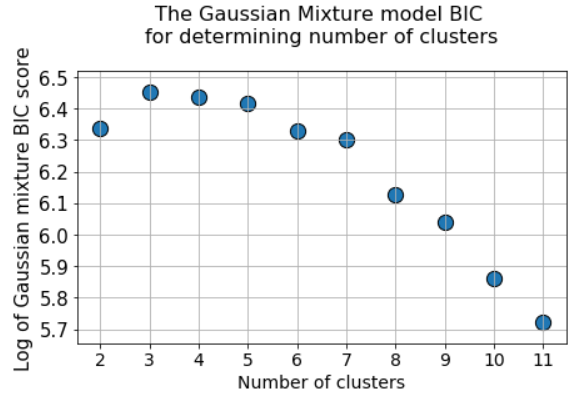
The BIC method fines numerous normal distributions and tries to keep the model simple enough to describe a given pattern.



Therefore, you can run the GMM algorithm for a large number of cluster centers, and the BIC value will increase to some point, and then begin to decline as the fine grows.

Total

Here is the Jupyter notebook for this article. Feel free to fork and experiment.



We at Jet Infosystems discussed a couple of alternatives to the popular elbow method in terms of choosing the right number of clusters when learning without a teacher using the k-means algorithm.



We made sure that instead of the elbow method, it is better to use the “silhouette” coefficient and the BIC value (from the GMM extension for k-means) to visually determine the optimal number of clusters.