Image Outline Detection Algorithms
The article presents the four most common loop detection algorithms.
The first two, namely the algorithm for tracing squares and tracing the surroundings of Moore, are easy to implement, and therefore are often used to determine the contour of a given pattern. Unfortunately, both algorithms have several weaknesses, which makes it impossible to detect the contour of a large class of patterns due to their special type of adjacency.
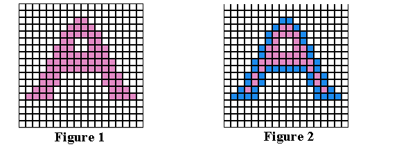
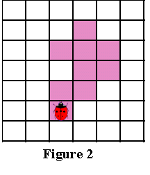
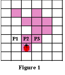
These algorithms will ignore all “holes” in the pattern. For example, if we have a pattern similar to that shown in Figure 1 , then the circuit detected by the algorithms will be similar to that shown in Figure 2 (the outline is indicated by blue pixels). In some areas of application this is quite acceptable, but in other areas, for example, in character recognition, detection of the internal parts of the pattern is required to find all the spaces that distinguish a specific character. ( Figure 3 shows the “full” outline of the pattern.)
Therefore, to obtain a complete contour, you must first use the “hole search” algorithm that determines the holes in a given pattern, and then apply the contour detection algorithm to each hole.

In digital images with binary values, a pixel can have one of the following values: 1 - when it is part of the pattern, or 0 - when it is part of the background, i.e. no gradation of gray. (We will assume that pixels with a value of 1 are black, and with a value of 0 are white).
To identify objects in a digital pattern, we need to find groups of black pixels that are “connected” to each other. In other words, the objects in a given digital pattern are the connected components of this pattern.
In the general case, a connected component is a set of black pixels P , such that for each pair of pixels p i and p j in P there is a sequence of pixels p i , ..., p j such that:
a) all the pixels in the sequence are in the set P , i.e. are black, and
b) every 2 pixels in the sequence adjacent are “neighbors”.
An important question arises: when can we say that 2 pixels are “neighbors”? Since we use square pixels, the answer to the previous question is not trivial for the following reason: in square tessellation, pixels have a common edge or a vertex, or have nothing in common. Each pixel has 8 pixels that share a vertex with it; such pixels make up the "Moore neighborhood" of that pixel. Should we consider “neighbors” pixels having only one common vertex? Or in order to be considered “neighbors”, two pixels must have a common edge?
So there are two types of connectivity, namely: 4-connectedness and 8-connectedness.
When can we say that a given set of black pixels is 4-connected? First, you need to define the concept of a 4-neighbor (also called a direct neighbor ):
4-neighbor definition : A pixel Q is a 4-neighbor of a given pixel P if Q and P have a common edge. The 4-neighbors of the pixel P (designated as P2, P4, P6, and P8 ) are shown in Figure 2 below.

Definition of a 4-connected component : the set of black pixels P is a 4-connected component if for each pair of pixels p i and p j in P there is a sequence of pixels p i , ..., p j such that:
a) all the pixels in the sequence are in the set P , i.e. are black, and
b) every two pixels that are adjacent in the sequence are 4 neighbors
The diagrams below show examples of 4-connected patterns:

When can I say that a given set of black pixels is 8-connected ? First, we need to define the concept of an 8-neighbor (also called an indirect neighbor ):
8-neighbor definition : A pixel Q is an 8-neighbor (or just a neighbor ) of a given pixel P if Q and P have a common edge or vertex. The 8-neighbors of a given pixel P make up the Moore neighborhood of this pixel.
Definition of an 8-connected component : the set of black pixels P is an 8-connected component (or just a connected component ) if for each pair of pixels p i and p j in P there is a sequence of pixels p i , ..., p j such that :
a) all the pixels in the sequence are in the set P , i.e. are black, and
b) every two pixels that are adjacent in this sequence are 8 neighbors
Note : all 4-connected patterns are 8-connected, i.e. 4-connected patterns are a subset of the many 8-connected patterns. On the other hand, an 8-connected pattern may not be 4-connected.
The diagram below shows a pattern that is 8-connected but not 4-connected:

The diagram below shows an example of a pattern that is not 8-connected, i.e. composed of more than one connected component (the diagram shows three connected components):

The idea behind the square trace algorithm is very simple; this can be attributed to the fact that the algorithm was one of the first attempts to detect the contour of a binary pattern.
To understand how it works, you need a little imagination ...
Suppose we have a digital pattern, for example, a group of black pixels on a background of white pixels, i.e. on the grid; find the black pixel and declare it as our " initial " pixel. (Finding the “ initial ” pixel can be implemented in many different ways; we will start from the lower left corner of the grid, we will scan each column of pixels from bottom to top, from the leftmost column to the rightmost, until we come across a black pixel. We will declare it “ initial ” ".)
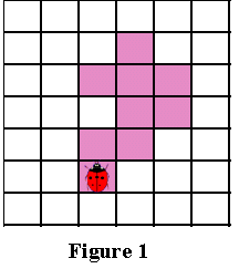
Now imagine that you are a ladybug standing on the starting pixel, as shown in Figure 1 below. To get the outline of a pattern, you need to do the following:
The black pixels that you circled will be the outline of the pattern.
An important aspect of the square trace algorithm is the “sense of direction”. Turns to the left and right are performed relative to the current location, which depends on how you got to the current pixel. Therefore, in order to make the right moves, you need to track your direction.
The following is a formal description of the square trace algorithm:
Input: square tessellation , T , containing the connected component P of black cells.
Output: row B (b 1 , b 2 , ..., b k ) of border pixels, i.e. circuit.
Start
the end
Note: the concepts of “left” and “right” should be considered not with respect to the page or reader, but with respect to the direction of entry into the “current” pixel during scanning.
The following is an animated demonstration of how the square trace algorithm detects the outline of a pattern. Do not forget that the ladybug moves in pixels; notice how its direction changes when turning left and right. Turns left and right are performed relative to the current direction in a pixel, i.e. ladybug orientations.
It turns out that the capabilities of the square trace algorithm are very limited. He is unable to detect the contours of a large family of patterns that often arise in real world applications.
This is mainly due to the fact that left and right rotations do not take into account pixels located “along
diagonals ”from the current pixel.
Let's look at the different patterns with different connectivity and see why the square trace algorithm fails. In addition, we will study ways to improve the capabilities of the algorithm and make it work even with patterns that have a special kind of connectivity.
One of the weaknesses of the algorithm is the choice of the stopping criterion. In other words, when does an algorithm stop executing?
In the original description of the square trace algorithm, the condition for completion is to hit the initial pixel a second time. It turns out that if the algorithm depends on such a criterion, then it will not be able to detect the contours of a large family of patterns.
The following is an animated demo explaining how the algorithm cannot detect the exact contour of the pattern due to the selection of a bad stopping criterion:
As you can see, improving the stopping criterion can be a good start to improve the overall performance of the algorithm. There are two effective alternatives for an existing shutdown criterion:
a) Stop only by visiting the starting pixel n times, where n is at least 2, OR
b) Stop after hitting the start pixel a second time, just like we hit it initially.
This criterion was proposed by Jacob Eliosoff , so we will call it the criterion for stopping Jacob .
Changing the stopping criterion generally improves the efficiency of the square trace algorithm, but does not allow to overcome other weaknesses that it has in the case of patterns with special types of connectivity.
Square Tracing Algorithm is unable to detect the contour of a family of patterns with a connectivity of 8 that does NOT have a connectivity of 4.
The following is an animated demonstration of how the square trace algorithm (with Jacob's stopping criterion) fails to detect the correct outline of a pattern with connectivity 8 without connectivity 4:
If you read the above analysis, you probably think that the square trace algorithm fails to detect the outlines of most patterns. But it turns out. that there is a special family of patterns in which the contour is fully detected by the square trace algorithm.
Let P be the set of black pixels with connectivity 4 on the grid. Let the white pixels of the grid, i.e. the background pixels W also have a connectivity of 4. It turns out that under such conditions of the pattern and its background, it can be proved that the square trace algorithm (with the Jacob stop criterion) will always successfully deal with the determination of the contour.
Below is the proof that in the case where both the pattern and the background pixels are 4 connected, the square trace algorithm will correctly determine the outline using the Jacob stop criterion.
Evidence
Given : the pattern P is such that all the pixels of the pattern (i.e. black) and the background pixels (i.e. white) W have a connectivity of 4.
First observation
Since the set of white pixels W has a connectivity of 4, this means that there cannot be any “ holes ” in the pattern (in informal terms, “ holes ” we mean groups of white pixels completely surrounded by black pixels of the pattern).
The presence of any “ hole ” in the pattern will lead to the separation of the group of white pixels from the remaining white pixels; while many white pixels lose their connectivity 4.
Figure 2 and Figure 3 below show two types of “ holes ” that can occur in a pattern with connectivity 4:

Second observation
Any two black pixels of a pattern MUST have one common side.
Suppose two black pixels have only one common vertex. Then, in order to satisfy the property of 4-connectedness of the pattern, there must be a path connecting these two pixels so that every two neighboring pixels on this path have a connectivity of 4. But this will give us a pattern similar to Figure 3 . In other words, this will result in white pixel separation. Figure 4 below shows a typical pattern satisfying the assumption that the pixels in the pattern and background are 4-connected, i.e. do not have “ holes ”, and every two black pixels have one common side:

It is useful to represent such patterns as follows:
First we consider the boundary pixels, i.e. outline of the pattern. Then, if we consider each boundary pixel as having 4 edges of unit length, we will see that some of these edges are common with neighboring white pixels. We call such edges boundary edges .
Such boundary edges can be considered as edges of a polygon. In the picture
5 below, this idea is demonstrated by the example of a polygon corresponding to the pattern from Figure 4 above:

If we consider all the possible “configurations” of boundary pixels that may occur in such patterns, then we will see that there are two simple cases, shown in Figure 6 and Figure 7 below.
The boundary pixels may be multiples of these cases or other arrangements, i.e. the twists and turns of these two cases. Boundary ribs are marked in blue as E1, E2, E3 and E4 .
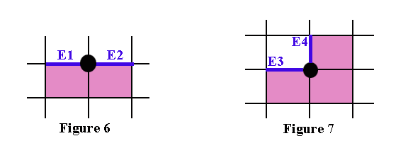
Third observation
In the case of the two cases discussed above, no matter which initial pixel we choose, and in whatever direction they fall into it, the square trace algorithm will never “go back” (backtrack) , will never “pass through” the boundary edge twice ( only if it does not trace the border a second time) and never miss the boundary edge . Check it out!
Two concepts need to be clarified here:
a) the algorithm “goes back” , when before tracing the entire border it goes back to visit an already visited pixel, and
b) for each boundary rib, there are two ways to “pass through it” , namely “inward” and “outward” (where “inward” means the movement inward of the corresponding polygon, and “outward” - outward of the polygon).
In addition, when the algorithm passes “inward” through one of the boundary edges, it will pass “outward” through the next boundary edge, i.e. the square trace algorithm should not be able to pass through two consecutive edges in the same way.
Last observation
Each pattern has an even number of boundary edges .
If you look at the polygon from Figure 5 , you can see that:
if we want to start from the vertex S marked in the diagram and follow the boundary edges until we reach S again, we notice that in the process we cross an even number of boundary edges. Each boundary rib can be considered a “step” in a separate direction. Then for each “step” to the right there must be a corresponding “step” to the left, if we want to return to the starting position. The same applies to vertical “steps.” Therefore, the “steps” must have corresponding pairs, and this explains why each of these patterns will have an even number of boundary edges.
Therefore, when the algorithm for tracing squares enters through the initial boundary edge (of the initial pixel) a second time, it will do it in the same direction as the first time.
The reason for this is that since there are two ways to go through the boundary edge, and the algorithm alternately moves inward and outward, and there are an even number of boundary edges, the algorithm will go through the initial boundary edge for the second time the same as in the first.
In the case of a 4-connected pattern and background, the square trace algorithm will detect the entire border, i.e. contour, pattern and will stop working after a single trace, i.e. It will not trace it again, because when it reaches the initial boundary edge for the second time, it will enter it the same way as the first time. Therefore, the square trace algorithm with Jacob's stop criterion will correctly determine the counter of any pattern, provided that both the pattern and the background are 4-connected.
The idea behind the Moore-Neighbor tracing is simple; but before explaining it, we need to explain an important concept: the Moore neighborhood of a pixel.
The Moore neighborhood of a pixel P is a set of 8 pixels having a common vertex or edge with that pixel. Such pixels, namely P1, P2, P3, P4, P5, P6, P7 and P8 , are shown in Figure 1 .
The Moore neighborhood (also called 8-neighbors or indirect neighbors ) is an important concept often referred to in the literature.

Now we are ready to get acquainted with the idea underlying the trace of the surroundings of Moore.
Let there be a digital pattern, i.e. a group of black pixels, on a background of white pixels, i.e. on the grid; find the black pixel and declare it the " initial " pixel. (There are several ways to find the “ initial ” pixel, but we, as before, will start from the lower left corner and scan all the columns of pixels in order, until we find the first black pixel, which we will declare to be the “ initial ”.)
Now again, imagine that you are a ladybug standing on the starting pixel, as shown in Figure 2 below. Without loss of generalization, we will detect the outline by moving around the pattern clockwise. (It does not matter which direction we choose, the main thing is to use it constantly in the algorithm).
The general idea is this: every time we get to the black pixel P , we go back, that is, to the white pixel in which we stood before. Then we go around the pixel P clockwise, visiting every pixel in its vicinity of Moore, until we get to the black pixel. The algorithm terminates when the starting pixel reaches the starting pixel a second time.
Those black pixels that the algorithm visited will be the outline of the pattern.
The following is a formal description of the Moore neighborhood tracing algorithm:
Input: square tessellation T containing a connected component P of black cells.
Output: row B (b 1 , b 2 , ..., b k ) of boundary pixels, i.e. circuit.
Denote by M (a) the Moore neighborhood of pixel a .
Let p be the current border pixel.
Let c be the current pixel under consideration, i.e. c is in M (p) .
Start
the end
The following is an animated demonstration of how Moore's neighborhood trace performs pattern outline detection. (We decided to trace the outline clockwise.)

The main weakness in tracing the surroundings of Moore lies in the choice of stopping criteria.
In the original description of the algorithm for tracing the surroundings of Moore, the stopping criterion is to hit the initial pixel a second time. Similar to the square tracing algorithm, it turns out that tracing the surroundings of Moore using this criterion cannot detect the contours of a large family of patterns.
The following is an animated demo explaining why the algorithm cannot find the exact outline of the pattern due to the selection of bad stopping criteria:

As you can see, improving the stopping criterion can be a good start to improving the overall performance of the trace. For the stop criterion, there are two effective alternatives similar to Jacob's stop criterion.
Using the Jacob criterion significantly improves the efficiency of tracing the surroundings of Moore, making it the best algorithm for determining the contour of any pattern, regardless of its connectivity.
The reason for this is mainly because the algorithm checks the entire Moore neighborhood of the boundary pixel to search for the next boundary pixel. Unlike the square trace algorithm, which only rotates left and right and misses the pixels “diagonally,” Moore’s neighborhood trace will always be able to detect the outer boundary of any connected component. The reason is this: for any 8-connected (or simply connected ) pattern, the next border pixel lies within the Moore neighborhood of the current border pixel. Since Moore's neighborhood trace checks each of the pixels in the Moore neighborhood of the current boundary pixel, it must detect the next boundary pixel.
When the tracing of the neighborhood of Moore reaches the initial pixel a second time in the same way as she did the first time, this means that a complete external contour of the pattern has been detected, and if the algorithm is not stopped, it will again detect the same contour.
The Radial Sweep Algorithm is a contour detection algorithm discussed in some books. Despite the complex name, the underlying idea is very simple. In fact, it turns out that the radial sweep algorithm is identical to the trace of Moore's surroundings. One may ask: “Why do we mention him at all?”
Tracing the surroundings of Moore searches in the vicinity of Moore for the current boundary pixel in a certain direction (we chose the clockwise direction) until it finds a black pixel. She then declares that pixel as the current boundary pixel and continues.
The radial scan algorithm does the same. On the other hand, it provides an interesting way to find the next black pixel in the Moore neighborhood of a given boundary pixel.
The method is based on the following idea:
every time we find a new border pixel, make it the current pixel P , and draw an imaginary line segment connecting P to the previous border pixel. Then rotate the segment relative to P clockwise until it comes across a black pixel in the Moore neighborhood of pixel P. The rotation of the line is identical to checking each pixel in the vicinity of Moore P.
We created an animated demonstration of how the radial scan algorithm works and how it looks like tracing the surroundings of Moore.

And when does the radial sweep algorithm stop?
Let's explain the behavior of the algorithm using the following stopping criteria ...
Let the radial scan algorithm complete when it visits the initial pixel a second time.
Below is an animated demo, from which it is clear why the break criterion will be changed correctly.

It is also worth mentioning that when using this stopping criterion in both algorithms, the effectiveness of the radial scan algorithm is identical to the tracing of Moore's surroundings.
In the square trace algorithm and in the Moore neighborhood trace, we found that using the Jacob stop criterion significantly improves the performance of both algorithms.
Jacob's stopping criterion requires the algorithm to stop executing when it visits the starting pixel a second time in the same direction as the first time.
Unfortunately, we cannot use the Jacob stop criterion in the radial sweep algorithm. The reason is that the radial scan algorithm does not define the conceptThe "direction" in which it hits the boundary pixel . In other words, it is not clear the “direction” in which the algorithm fell into the boundary pixel (and its definition is nontrivial).
Therefore, we need to propose another stopping criterion, which does not depend on the direction of hitting a certain pixel, which can improve the effectiveness of the radial scan algorithm ...
Suppose that each time the algorithm detects a new boundary pixel P i , it is inserted into a series of boundary pixels: P 1 , P 2 , P 3 , ..., P i ; and declared as the current border pixel. ( P 1 we will consider the initial pixel). This means that we know the previous border pixel P i-1 of each current border pixel P i . (As for the starting pixel , we will assume that P 0is an imaginary pixel that is nonequivalent to any of the pixels on the grid that faces the initial pixel in the row of boundary pixels).
Based on the above assumptions, we can determine the stopping criterion as follows:
The algorithm stops execution when:
a) the current boundary pixel P i has previously met as a pixel P j (where j <i ) in a series of boundary pixels, And
b) P i- 1 = P j-1 .
In other words, the algorithm completes execution when it visits the boundary pixel P in the secondtimes if the boundary pixel before P (in the row of boundary pixels) for the second time is the same pixel as it was before P when P was visited for the first time.
If the condition of the stop criterion is satisfied and the algorithm does not shut down, then the radial scan algorithm will continue to detect the same boundary a second time.
The effectiveness of the radial scan algorithm with this stopping criterion is similar to the performance of tracing the Moore neighborhood with the Jacob stopping criterion.
This algorithm is one of the latest loop detection algorithms proposed by Theo Pavlidis . He cited it in his 1982 book Algorithms for Graphics and Image Processing (chapter 7, section 5). It is not so simple as the algorithm for tracing squares or tracing the surroundings of Moore, but it is not so complicated (this is characteristic of most contour detection algorithms).
We will not explain this algorithm in the way it was done in his book. Our approach is easier to understand and gives an idea of the general idea underlying the algorithm.
Without loss of generalization, we decided to go around the loop clockwise to match the order of all the other algorithms presented in the article. On the other hand, Pavlidis chose the direction counterclockwise. This will not affect the performance of the algorithm. The only difference is the relative direction of the movements that we will do when we go around the contour.
Now let's move on to the idea ...
Let's say we have a digital pattern, i.e. a group of black pixels on a background of white pixels, i.e. on the grid; find the black pixel and declare it the " initial " pixel. You can search for the “ starting ” pixel in various ways, for example, as described above.
To find the initialpixels to use this method is optional. Instead, we will choose a starting pixel that satisfies the following restrictions imposed by the Pavlidis algorithm for choosing a starting pixel:
An important limitation of the direction in which we enter the starting pixel
In fact, you can choose ANY black border pixel as the starting pixel under this condition: if you initially stand on it, the left neighboring pixel is NOT black. In other words, you need to enter the initial pixel in such a direction that the left neighboring pixel is white (the “left” here is taken relative to the direction in which we enter the initial pixel ).
Now imagine that you are a ladybug standing onstarting pixel, as shown in Figure 1 below. In the process of executing the algorithm, we will be interested in only three pixels in front of you, i.e. P1, P2 and P3 shown in Figure 1 . (We will designate P2 as the pixel in front of you, P1 is the pixel to the left of P2 , and P3 is the pixel to the right of P2 ).
As with the square trace algorithm, the most important thing in the Pavlidis algorithm is the “sense of direction”. Turns left and right are performed relative to the current position, which depends on how you entered the current pixel. Therefore, in order to make the right moves, it is important to keep track of your current orientation. But no matter how you are located, the pixels P1, P2 and P3 are determined as described above.
Having this information, we are ready to explain the algorithm ...
Each time you are standing on the current boundary pixel (which is first the initial pixel), we do the following:
First , check the pixel P1 . If P1 is black, then declare P1the current boundary pixel and move one step forward, and then take a step to the left to be on P1 (the order of moves is very important).
In Figure 2 below illustrates this case. The path to get to P1 is shown in blue.

And only if P1 is white, we proceed to check P2 ...
If P2 is black, then declare P2 the current boundary pixel and move one step forward to be on P2 . This case is shown in Figure 3 below. The path you need to follow on P2 is shown in blue.

Only if both P1 and P2 are white, go to check P3 ...
If P3 is black, then declare P3 the current border pixel and move one step to the right, and then one step to the left , as shown in Figure 4 below.
That's all! Three simple rules for three simple cases. As you can see, it is important to keep track of your direction when cornering, because all moves are made relative to the current orientation. But it seems we forgot something? What if all three pixels are white in front of us? Then we rotate (standing at the current boundary pixel) 90 degrees clockwise to see a new set of three pixels in front of us. Then we do the same check for these new pixels. You may still have a question: what if all these three pixels are white ?! Then again we turn 90 degrees clockwise, standing at the same pixel. Before you check the entire neighborhood of Moore's pixel, you can rotate three times (each time 90 degrees clockwise).
If we rotate three times without ever finding black pixels, then this means that we are standing on an isolated pixel that is not connected to any other black pixel. That is why the algorithm allows you to rotate three times, and then completes its execution.
Another aspect: When does the algorithm complete execution?
The algorithm completes the work in two cases:
a) as mentioned above. the algorithm allows you to rotate three times (90 degrees clockwise each time), after it completes the execution and declares the pixel isolated OR
b) when the current boundary pixel is the initial pixel, the algorithm completes the execution by “declaring” that it detected the pattern outline.
The following is a formal description of the Pavlidis algorithm:
Input: square tessellation T containing a connected component P of black cells.
Output: row B (b 1 , b 2 , ..., b k ) of boundary pixels, i.e. circuit.
Definitions:
Start
the end
The following is an animated demonstration of how the Pavlidis algorithm detects the contour of a given pattern. Do not forget that we walk in pixels; notice how the orientation changes when turning left or right. To explain the algorithm in as much detail as possible, we included all possible cases in it.
If you think that the Pavlidis algorithm is ideal for detecting pattern outlines, then you should change your mind ...
This algorithm is really a little more complicated than, for example, tracing the surroundings of Moore, in which there are no special cases that require separate processing, but he will not be able to determine the outlines of a large a family of patterns that has a certain kind of connectivity.
The algorithm works very well on 4-connected patterns. Its problem occurs when tracing some 8-connected patterns that are not 4-connected. The following is an animated demonstration of how the Pavlidis algorithm fails to detect the correct outline of an 8-connected pattern (not a 4-connected one) - it skips most of the border.
There are two simple ways to modify an algorithm to significantly improve its performance.
a) Replace the stop criterion
Instead of completing the algorithm when it visits the start pixel a second time, you can end it when it visits the start pixel a third or even fourth time. This will improve the overall performance of the algorithm.
OR
b) Get to the source of the problem, namely, before choosing the starting pixel.
There is an important limitation regarding the direction in which the entry to the starting pixel is performed. Essentially, you need to enter the starting pixel so that when you stand on it, the pixel to your left is white. The reason for introducing this restriction is this: since we always look at the three pixels in front of us in a certain order , in some patterns we will skip the boundary pixel that lies directly to the left of the initial pixel.
We risk missing not only the left neighboring pixel from the starting pixel, but also the pixel directly below it(as demonstrated in the analysis). In addition, in some patterns, a pixel corresponding to the pixel R in Figure 5 below will be skipped . Therefore, we assume that the starting pixel needs to be hit in such a direction that the pixels corresponding to the pixels L, W and R shown in Figure 5 below are white.
In this case, patterns like the one shown in the demonstration will be detected correctly and the effectiveness of the Pavlidis algorithm will improve significantly. On the other hand, finding an initial pixel that satisfies these requirements can be a difficult task, and in many cases it will be impossible to find such a pixel. In this case, you should use an alternative way to improve the Pavlidis algorithm, namely the completion of the algorithm after visiting the starting point for the third time.
The first two, namely the algorithm for tracing squares and tracing the surroundings of Moore, are easy to implement, and therefore are often used to determine the contour of a given pattern. Unfortunately, both algorithms have several weaknesses, which makes it impossible to detect the contour of a large class of patterns due to their special type of adjacency.
These algorithms will ignore all “holes” in the pattern. For example, if we have a pattern similar to that shown in Figure 1 , then the circuit detected by the algorithms will be similar to that shown in Figure 2 (the outline is indicated by blue pixels). In some areas of application this is quite acceptable, but in other areas, for example, in character recognition, detection of the internal parts of the pattern is required to find all the spaces that distinguish a specific character. ( Figure 3 shows the “full” outline of the pattern.)
Therefore, to obtain a complete contour, you must first use the “hole search” algorithm that determines the holes in a given pattern, and then apply the contour detection algorithm to each hole.
What is connectivity?
In digital images with binary values, a pixel can have one of the following values: 1 - when it is part of the pattern, or 0 - when it is part of the background, i.e. no gradation of gray. (We will assume that pixels with a value of 1 are black, and with a value of 0 are white).
To identify objects in a digital pattern, we need to find groups of black pixels that are “connected” to each other. In other words, the objects in a given digital pattern are the connected components of this pattern.
In the general case, a connected component is a set of black pixels P , such that for each pair of pixels p i and p j in P there is a sequence of pixels p i , ..., p j such that:
a) all the pixels in the sequence are in the set P , i.e. are black, and
b) every 2 pixels in the sequence adjacent are “neighbors”.
An important question arises: when can we say that 2 pixels are “neighbors”? Since we use square pixels, the answer to the previous question is not trivial for the following reason: in square tessellation, pixels have a common edge or a vertex, or have nothing in common. Each pixel has 8 pixels that share a vertex with it; such pixels make up the "Moore neighborhood" of that pixel. Should we consider “neighbors” pixels having only one common vertex? Or in order to be considered “neighbors”, two pixels must have a common edge?
So there are two types of connectivity, namely: 4-connectedness and 8-connectedness.
4-connection
When can we say that a given set of black pixels is 4-connected? First, you need to define the concept of a 4-neighbor (also called a direct neighbor ):
4-neighbor definition : A pixel Q is a 4-neighbor of a given pixel P if Q and P have a common edge. The 4-neighbors of the pixel P (designated as P2, P4, P6, and P8 ) are shown in Figure 2 below.
Definition of a 4-connected component : the set of black pixels P is a 4-connected component if for each pair of pixels p i and p j in P there is a sequence of pixels p i , ..., p j such that:
a) all the pixels in the sequence are in the set P , i.e. are black, and
b) every two pixels that are adjacent in the sequence are 4 neighbors
Examples of 4-connected patterns
The diagrams below show examples of 4-connected patterns:
8-connection
When can I say that a given set of black pixels is 8-connected ? First, we need to define the concept of an 8-neighbor (also called an indirect neighbor ):
8-neighbor definition : A pixel Q is an 8-neighbor (or just a neighbor ) of a given pixel P if Q and P have a common edge or vertex. The 8-neighbors of a given pixel P make up the Moore neighborhood of this pixel.
Definition of an 8-connected component : the set of black pixels P is an 8-connected component (or just a connected component ) if for each pair of pixels p i and p j in P there is a sequence of pixels p i , ..., p j such that :
a) all the pixels in the sequence are in the set P , i.e. are black, and
b) every two pixels that are adjacent in this sequence are 8 neighbors
Note : all 4-connected patterns are 8-connected, i.e. 4-connected patterns are a subset of the many 8-connected patterns. On the other hand, an 8-connected pattern may not be 4-connected.
8-linked pattern example
The diagram below shows a pattern that is 8-connected but not 4-connected:
An example of a non-8-connected pattern:
The diagram below shows an example of a pattern that is not 8-connected, i.e. composed of more than one connected component (the diagram shows three connected components):
Square Trace Algorithm
Idea
The idea behind the square trace algorithm is very simple; this can be attributed to the fact that the algorithm was one of the first attempts to detect the contour of a binary pattern.
To understand how it works, you need a little imagination ...
Suppose we have a digital pattern, for example, a group of black pixels on a background of white pixels, i.e. on the grid; find the black pixel and declare it as our " initial " pixel. (Finding the “ initial ” pixel can be implemented in many different ways; we will start from the lower left corner of the grid, we will scan each column of pixels from bottom to top, from the leftmost column to the rightmost, until we come across a black pixel. We will declare it “ initial ” ".)
Now imagine that you are a ladybug standing on the starting pixel, as shown in Figure 1 below. To get the outline of a pattern, you need to do the following:
, , ,
, , ,
.
The black pixels that you circled will be the outline of the pattern.
An important aspect of the square trace algorithm is the “sense of direction”. Turns to the left and right are performed relative to the current location, which depends on how you got to the current pixel. Therefore, in order to make the right moves, you need to track your direction.
Algorithm
The following is a formal description of the square trace algorithm:
Input: square tessellation , T , containing the connected component P of black cells.
Output: row B (b 1 , b 2 , ..., b k ) of border pixels, i.e. circuit.
Start
- Define B as an empty set.
- We scan cells T from bottom to top and left to right until a black pixel s from P is found .
- Insert s into B.
- Make the current pixel p the initial pixel s .
- Turn left, i.e. go to the neighboring pixel to the left of p .
- Update p , i.e. it becomes the current pixel.
- While p is not equal to s , execute
If the current pixel p is black
- insert p into B and turn left (go to the neighboring pixel to the left of p ).
- Update p , i.e. it becomes the current pixel.
otherwise
- turn right (go to the neighboring pixel to the right of p ).
- Update p , i.e. it becomes the current pixel.
End of the “Bye” cycle
the end
Note: the concepts of “left” and “right” should be considered not with respect to the page or reader, but with respect to the direction of entry into the “current” pixel during scanning.
Demonstration
The following is an animated demonstration of how the square trace algorithm detects the outline of a pattern. Do not forget that the ladybug moves in pixels; notice how its direction changes when turning left and right. Turns left and right are performed relative to the current direction in a pixel, i.e. ladybug orientations.
Analysis
It turns out that the capabilities of the square trace algorithm are very limited. He is unable to detect the contours of a large family of patterns that often arise in real world applications.
This is mainly due to the fact that left and right rotations do not take into account pixels located “along
diagonals ”from the current pixel.
Let's look at the different patterns with different connectivity and see why the square trace algorithm fails. In addition, we will study ways to improve the capabilities of the algorithm and make it work even with patterns that have a special kind of connectivity.
Stop criterion
One of the weaknesses of the algorithm is the choice of the stopping criterion. In other words, when does an algorithm stop executing?
In the original description of the square trace algorithm, the condition for completion is to hit the initial pixel a second time. It turns out that if the algorithm depends on such a criterion, then it will not be able to detect the contours of a large family of patterns.
The following is an animated demo explaining how the algorithm cannot detect the exact contour of the pattern due to the selection of a bad stopping criterion:
As you can see, improving the stopping criterion can be a good start to improve the overall performance of the algorithm. There are two effective alternatives for an existing shutdown criterion:
a) Stop only by visiting the starting pixel n times, where n is at least 2, OR
b) Stop after hitting the start pixel a second time, just like we hit it initially.
This criterion was proposed by Jacob Eliosoff , so we will call it the criterion for stopping Jacob .
Changing the stopping criterion generally improves the efficiency of the square trace algorithm, but does not allow to overcome other weaknesses that it has in the case of patterns with special types of connectivity.
Square Tracing Algorithm is unable to detect the contour of a family of patterns with a connectivity of 8 that does NOT have a connectivity of 4.
The following is an animated demonstration of how the square trace algorithm (with Jacob's stopping criterion) fails to detect the correct outline of a pattern with connectivity 8 without connectivity 4:
Is this algorithm completely useless?
If you read the above analysis, you probably think that the square trace algorithm fails to detect the outlines of most patterns. But it turns out. that there is a special family of patterns in which the contour is fully detected by the square trace algorithm.
Let P be the set of black pixels with connectivity 4 on the grid. Let the white pixels of the grid, i.e. the background pixels W also have a connectivity of 4. It turns out that under such conditions of the pattern and its background, it can be proved that the square trace algorithm (with the Jacob stop criterion) will always successfully deal with the determination of the contour.
Below is the proof that in the case where both the pattern and the background pixels are 4 connected, the square trace algorithm will correctly determine the outline using the Jacob stop criterion.
Evidence
Given : the pattern P is such that all the pixels of the pattern (i.e. black) and the background pixels (i.e. white) W have a connectivity of 4.
First observation
Since the set of white pixels W has a connectivity of 4, this means that there cannot be any “ holes ” in the pattern (in informal terms, “ holes ” we mean groups of white pixels completely surrounded by black pixels of the pattern).
The presence of any “ hole ” in the pattern will lead to the separation of the group of white pixels from the remaining white pixels; while many white pixels lose their connectivity 4.
Figure 2 and Figure 3 below show two types of “ holes ” that can occur in a pattern with connectivity 4:
Second observation
Any two black pixels of a pattern MUST have one common side.
Suppose two black pixels have only one common vertex. Then, in order to satisfy the property of 4-connectedness of the pattern, there must be a path connecting these two pixels so that every two neighboring pixels on this path have a connectivity of 4. But this will give us a pattern similar to Figure 3 . In other words, this will result in white pixel separation. Figure 4 below shows a typical pattern satisfying the assumption that the pixels in the pattern and background are 4-connected, i.e. do not have “ holes ”, and every two black pixels have one common side:
It is useful to represent such patterns as follows:
First we consider the boundary pixels, i.e. outline of the pattern. Then, if we consider each boundary pixel as having 4 edges of unit length, we will see that some of these edges are common with neighboring white pixels. We call such edges boundary edges .
Such boundary edges can be considered as edges of a polygon. In the picture
5 below, this idea is demonstrated by the example of a polygon corresponding to the pattern from Figure 4 above:
If we consider all the possible “configurations” of boundary pixels that may occur in such patterns, then we will see that there are two simple cases, shown in Figure 6 and Figure 7 below.
The boundary pixels may be multiples of these cases or other arrangements, i.e. the twists and turns of these two cases. Boundary ribs are marked in blue as E1, E2, E3 and E4 .
Third observation
In the case of the two cases discussed above, no matter which initial pixel we choose, and in whatever direction they fall into it, the square trace algorithm will never “go back” (backtrack) , will never “pass through” the boundary edge twice ( only if it does not trace the border a second time) and never miss the boundary edge . Check it out!
Two concepts need to be clarified here:
a) the algorithm “goes back” , when before tracing the entire border it goes back to visit an already visited pixel, and
b) for each boundary rib, there are two ways to “pass through it” , namely “inward” and “outward” (where “inward” means the movement inward of the corresponding polygon, and “outward” - outward of the polygon).
In addition, when the algorithm passes “inward” through one of the boundary edges, it will pass “outward” through the next boundary edge, i.e. the square trace algorithm should not be able to pass through two consecutive edges in the same way.
Last observation
Each pattern has an even number of boundary edges .
If you look at the polygon from Figure 5 , you can see that:
if we want to start from the vertex S marked in the diagram and follow the boundary edges until we reach S again, we notice that in the process we cross an even number of boundary edges. Each boundary rib can be considered a “step” in a separate direction. Then for each “step” to the right there must be a corresponding “step” to the left, if we want to return to the starting position. The same applies to vertical “steps.” Therefore, the “steps” must have corresponding pairs, and this explains why each of these patterns will have an even number of boundary edges.
Therefore, when the algorithm for tracing squares enters through the initial boundary edge (of the initial pixel) a second time, it will do it in the same direction as the first time.
The reason for this is that since there are two ways to go through the boundary edge, and the algorithm alternately moves inward and outward, and there are an even number of boundary edges, the algorithm will go through the initial boundary edge for the second time the same as in the first.
Conclusion
In the case of a 4-connected pattern and background, the square trace algorithm will detect the entire border, i.e. contour, pattern and will stop working after a single trace, i.e. It will not trace it again, because when it reaches the initial boundary edge for the second time, it will enter it the same way as the first time. Therefore, the square trace algorithm with Jacob's stop criterion will correctly determine the counter of any pattern, provided that both the pattern and the background are 4-connected.
Tracing the surroundings of Moore
Idea
The idea behind the Moore-Neighbor tracing is simple; but before explaining it, we need to explain an important concept: the Moore neighborhood of a pixel.
Neighborhood of Moore
The Moore neighborhood of a pixel P is a set of 8 pixels having a common vertex or edge with that pixel. Such pixels, namely P1, P2, P3, P4, P5, P6, P7 and P8 , are shown in Figure 1 .
The Moore neighborhood (also called 8-neighbors or indirect neighbors ) is an important concept often referred to in the literature.
Now we are ready to get acquainted with the idea underlying the trace of the surroundings of Moore.
Let there be a digital pattern, i.e. a group of black pixels, on a background of white pixels, i.e. on the grid; find the black pixel and declare it the " initial " pixel. (There are several ways to find the “ initial ” pixel, but we, as before, will start from the lower left corner and scan all the columns of pixels in order, until we find the first black pixel, which we will declare to be the “ initial ”.)
Now again, imagine that you are a ladybug standing on the starting pixel, as shown in Figure 2 below. Without loss of generalization, we will detect the outline by moving around the pattern clockwise. (It does not matter which direction we choose, the main thing is to use it constantly in the algorithm).
The general idea is this: every time we get to the black pixel P , we go back, that is, to the white pixel in which we stood before. Then we go around the pixel P clockwise, visiting every pixel in its vicinity of Moore, until we get to the black pixel. The algorithm terminates when the starting pixel reaches the starting pixel a second time.
Those black pixels that the algorithm visited will be the outline of the pattern.
Algorithm
The following is a formal description of the Moore neighborhood tracing algorithm:
Input: square tessellation T containing a connected component P of black cells.
Output: row B (b 1 , b 2 , ..., b k ) of boundary pixels, i.e. circuit.
Denote by M (a) the Moore neighborhood of pixel a .
Let p be the current border pixel.
Let c be the current pixel under consideration, i.e. c is in M (p) .
Start
- Define B as an empty set.
- From bottom to top and from left to right, scan cells T until we find a black pixel s from P.
- Insert s into B.
- Let us set the point s as the current boundary point p , i.e. p = s
- Let's go back, i.e. let's move on to the pixel from which we came to s .
- Let c be the next clockwise pixel in M (p) .
- While c is not equal to s , execute
- if c is black
- Insert c into B
- we set p = c
- go back (move the current pixel c to the pixel from which we got to p )
otherwise
- move the current pixel c to the next clockwise pixel in M (p)
End of the Bye Cycle
- if c is black
the end
Demonstration
The following is an animated demonstration of how Moore's neighborhood trace performs pattern outline detection. (We decided to trace the outline clockwise.)
Analysis
The main weakness in tracing the surroundings of Moore lies in the choice of stopping criteria.
In the original description of the algorithm for tracing the surroundings of Moore, the stopping criterion is to hit the initial pixel a second time. Similar to the square tracing algorithm, it turns out that tracing the surroundings of Moore using this criterion cannot detect the contours of a large family of patterns.
The following is an animated demo explaining why the algorithm cannot find the exact outline of the pattern due to the selection of bad stopping criteria:
As you can see, improving the stopping criterion can be a good start to improving the overall performance of the trace. For the stop criterion, there are two effective alternatives similar to Jacob's stop criterion.
Using the Jacob criterion significantly improves the efficiency of tracing the surroundings of Moore, making it the best algorithm for determining the contour of any pattern, regardless of its connectivity.
The reason for this is mainly because the algorithm checks the entire Moore neighborhood of the boundary pixel to search for the next boundary pixel. Unlike the square trace algorithm, which only rotates left and right and misses the pixels “diagonally,” Moore’s neighborhood trace will always be able to detect the outer boundary of any connected component. The reason is this: for any 8-connected (or simply connected ) pattern, the next border pixel lies within the Moore neighborhood of the current border pixel. Since Moore's neighborhood trace checks each of the pixels in the Moore neighborhood of the current boundary pixel, it must detect the next boundary pixel.
When the tracing of the neighborhood of Moore reaches the initial pixel a second time in the same way as she did the first time, this means that a complete external contour of the pattern has been detected, and if the algorithm is not stopped, it will again detect the same contour.
Radial scan
The Radial Sweep Algorithm is a contour detection algorithm discussed in some books. Despite the complex name, the underlying idea is very simple. In fact, it turns out that the radial sweep algorithm is identical to the trace of Moore's surroundings. One may ask: “Why do we mention him at all?”
Tracing the surroundings of Moore searches in the vicinity of Moore for the current boundary pixel in a certain direction (we chose the clockwise direction) until it finds a black pixel. She then declares that pixel as the current boundary pixel and continues.
The radial scan algorithm does the same. On the other hand, it provides an interesting way to find the next black pixel in the Moore neighborhood of a given boundary pixel.
The method is based on the following idea:
every time we find a new border pixel, make it the current pixel P , and draw an imaginary line segment connecting P to the previous border pixel. Then rotate the segment relative to P clockwise until it comes across a black pixel in the Moore neighborhood of pixel P. The rotation of the line is identical to checking each pixel in the vicinity of Moore P.
We created an animated demonstration of how the radial scan algorithm works and how it looks like tracing the surroundings of Moore.
And when does the radial sweep algorithm stop?
Let's explain the behavior of the algorithm using the following stopping criteria ...
Stop criterion 1
Let the radial scan algorithm complete when it visits the initial pixel a second time.
Below is an animated demo, from which it is clear why the break criterion will be changed correctly.
It is also worth mentioning that when using this stopping criterion in both algorithms, the effectiveness of the radial scan algorithm is identical to the tracing of Moore's surroundings.
In the square trace algorithm and in the Moore neighborhood trace, we found that using the Jacob stop criterion significantly improves the performance of both algorithms.
Jacob's stopping criterion requires the algorithm to stop executing when it visits the starting pixel a second time in the same direction as the first time.
Unfortunately, we cannot use the Jacob stop criterion in the radial sweep algorithm. The reason is that the radial scan algorithm does not define the conceptThe "direction" in which it hits the boundary pixel . In other words, it is not clear the “direction” in which the algorithm fell into the boundary pixel (and its definition is nontrivial).
Therefore, we need to propose another stopping criterion, which does not depend on the direction of hitting a certain pixel, which can improve the effectiveness of the radial scan algorithm ...
Stop criterion 2
Suppose that each time the algorithm detects a new boundary pixel P i , it is inserted into a series of boundary pixels: P 1 , P 2 , P 3 , ..., P i ; and declared as the current border pixel. ( P 1 we will consider the initial pixel). This means that we know the previous border pixel P i-1 of each current border pixel P i . (As for the starting pixel , we will assume that P 0is an imaginary pixel that is nonequivalent to any of the pixels on the grid that faces the initial pixel in the row of boundary pixels).
Based on the above assumptions, we can determine the stopping criterion as follows:
The algorithm stops execution when:
a) the current boundary pixel P i has previously met as a pixel P j (where j <i ) in a series of boundary pixels, And
b) P i- 1 = P j-1 .
In other words, the algorithm completes execution when it visits the boundary pixel P in the secondtimes if the boundary pixel before P (in the row of boundary pixels) for the second time is the same pixel as it was before P when P was visited for the first time.
If the condition of the stop criterion is satisfied and the algorithm does not shut down, then the radial scan algorithm will continue to detect the same boundary a second time.
The effectiveness of the radial scan algorithm with this stopping criterion is similar to the performance of tracing the Moore neighborhood with the Jacob stopping criterion.
Theo Pavlidis Algorithm
Idea
This algorithm is one of the latest loop detection algorithms proposed by Theo Pavlidis . He cited it in his 1982 book Algorithms for Graphics and Image Processing (chapter 7, section 5). It is not so simple as the algorithm for tracing squares or tracing the surroundings of Moore, but it is not so complicated (this is characteristic of most contour detection algorithms).
We will not explain this algorithm in the way it was done in his book. Our approach is easier to understand and gives an idea of the general idea underlying the algorithm.
Without loss of generalization, we decided to go around the loop clockwise to match the order of all the other algorithms presented in the article. On the other hand, Pavlidis chose the direction counterclockwise. This will not affect the performance of the algorithm. The only difference is the relative direction of the movements that we will do when we go around the contour.
Now let's move on to the idea ...
Let's say we have a digital pattern, i.e. a group of black pixels on a background of white pixels, i.e. on the grid; find the black pixel and declare it the " initial " pixel. You can search for the “ starting ” pixel in various ways, for example, as described above.
To find the initialpixels to use this method is optional. Instead, we will choose a starting pixel that satisfies the following restrictions imposed by the Pavlidis algorithm for choosing a starting pixel:
An important limitation of the direction in which we enter the starting pixel
In fact, you can choose ANY black border pixel as the starting pixel under this condition: if you initially stand on it, the left neighboring pixel is NOT black. In other words, you need to enter the initial pixel in such a direction that the left neighboring pixel is white (the “left” here is taken relative to the direction in which we enter the initial pixel ).
Now imagine that you are a ladybug standing onstarting pixel, as shown in Figure 1 below. In the process of executing the algorithm, we will be interested in only three pixels in front of you, i.e. P1, P2 and P3 shown in Figure 1 . (We will designate P2 as the pixel in front of you, P1 is the pixel to the left of P2 , and P3 is the pixel to the right of P2 ).
As with the square trace algorithm, the most important thing in the Pavlidis algorithm is the “sense of direction”. Turns left and right are performed relative to the current position, which depends on how you entered the current pixel. Therefore, in order to make the right moves, it is important to keep track of your current orientation. But no matter how you are located, the pixels P1, P2 and P3 are determined as described above.
Having this information, we are ready to explain the algorithm ...
Each time you are standing on the current boundary pixel (which is first the initial pixel), we do the following:
First , check the pixel P1 . If P1 is black, then declare P1the current boundary pixel and move one step forward, and then take a step to the left to be on P1 (the order of moves is very important).
In Figure 2 below illustrates this case. The path to get to P1 is shown in blue.
And only if P1 is white, we proceed to check P2 ...
If P2 is black, then declare P2 the current boundary pixel and move one step forward to be on P2 . This case is shown in Figure 3 below. The path you need to follow on P2 is shown in blue.
Only if both P1 and P2 are white, go to check P3 ...
If P3 is black, then declare P3 the current border pixel and move one step to the right, and then one step to the left , as shown in Figure 4 below.
That's all! Three simple rules for three simple cases. As you can see, it is important to keep track of your direction when cornering, because all moves are made relative to the current orientation. But it seems we forgot something? What if all three pixels are white in front of us? Then we rotate (standing at the current boundary pixel) 90 degrees clockwise to see a new set of three pixels in front of us. Then we do the same check for these new pixels. You may still have a question: what if all these three pixels are white ?! Then again we turn 90 degrees clockwise, standing at the same pixel. Before you check the entire neighborhood of Moore's pixel, you can rotate three times (each time 90 degrees clockwise).
If we rotate three times without ever finding black pixels, then this means that we are standing on an isolated pixel that is not connected to any other black pixel. That is why the algorithm allows you to rotate three times, and then completes its execution.
Another aspect: When does the algorithm complete execution?
The algorithm completes the work in two cases:
a) as mentioned above. the algorithm allows you to rotate three times (90 degrees clockwise each time), after it completes the execution and declares the pixel isolated OR
b) when the current boundary pixel is the initial pixel, the algorithm completes the execution by “declaring” that it detected the pattern outline.
Algorithm
The following is a formal description of the Pavlidis algorithm:
Input: square tessellation T containing a connected component P of black cells.
Output: row B (b 1 , b 2 , ..., b k ) of boundary pixels, i.e. circuit.
Definitions:
- Denote by p the current boundary pixel, i.e. the pixel on which we stand.
- Define P1, P2, and P3 as follows: (see also Figure 1 above)
- P2 is the pixel in front of you, adjacent to the one you are standing on, i.e. with pixel p .
- P1 — , P2 .
- P3 — , P2 .
- «» .
Start
- B .
- T , s P (. , )
- s B .
- p s .
- :
P1
- P1 B
- p=P1
- ,
P2
- P2 B
- p=P2
- (. 3)
P3
- P3 B
- p=P3
- , (. 4)
90 , p
- terminate the program and declare p an isolated pixel
otherwise
- rotate 90 degrees clockwise, standing at the current pixel p
While p = s (Finish the repeat loop)
the end
Demonstration
The following is an animated demonstration of how the Pavlidis algorithm detects the contour of a given pattern. Do not forget that we walk in pixels; notice how the orientation changes when turning left or right. To explain the algorithm in as much detail as possible, we included all possible cases in it.
Analysis
If you think that the Pavlidis algorithm is ideal for detecting pattern outlines, then you should change your mind ...
This algorithm is really a little more complicated than, for example, tracing the surroundings of Moore, in which there are no special cases that require separate processing, but he will not be able to determine the outlines of a large a family of patterns that has a certain kind of connectivity.
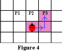
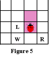
The algorithm works very well on 4-connected patterns. Its problem occurs when tracing some 8-connected patterns that are not 4-connected. The following is an animated demonstration of how the Pavlidis algorithm fails to detect the correct outline of an 8-connected pattern (not a 4-connected one) - it skips most of the border.
There are two simple ways to modify an algorithm to significantly improve its performance.
a) Replace the stop criterion
Instead of completing the algorithm when it visits the start pixel a second time, you can end it when it visits the start pixel a third or even fourth time. This will improve the overall performance of the algorithm.
OR
b) Get to the source of the problem, namely, before choosing the starting pixel.
There is an important limitation regarding the direction in which the entry to the starting pixel is performed. Essentially, you need to enter the starting pixel so that when you stand on it, the pixel to your left is white. The reason for introducing this restriction is this: since we always look at the three pixels in front of us in a certain order , in some patterns we will skip the boundary pixel that lies directly to the left of the initial pixel.
We risk missing not only the left neighboring pixel from the starting pixel, but also the pixel directly below it(as demonstrated in the analysis). In addition, in some patterns, a pixel corresponding to the pixel R in Figure 5 below will be skipped . Therefore, we assume that the starting pixel needs to be hit in such a direction that the pixels corresponding to the pixels L, W and R shown in Figure 5 below are white.
In this case, patterns like the one shown in the demonstration will be detected correctly and the effectiveness of the Pavlidis algorithm will improve significantly. On the other hand, finding an initial pixel that satisfies these requirements can be a difficult task, and in many cases it will be impossible to find such a pixel. In this case, you should use an alternative way to improve the Pavlidis algorithm, namely the completion of the algorithm after visiting the starting point for the third time.
All Articles