3D rendering using OpenGL

Introduction

What is OpenGL?

OpenGL is a specification that defines a platform-independent software interface for writing applications using two-dimensional and three-dimensional computer graphics. OpenGL is not an implementation, but only describes those sets of instructions that should be implemented, i.e. is an API.

Each version of OpenGL has its own specification, we will work from version 3.3 to version 4.6, because all innovations from version 3.3 affect aspects that are of little significance to us. Before you start writing your first OpenGL application, I recommend that you find out which versions your driver supports (you can do this on the vendor’s website of your video card) and update the driver to the latest version.

OpenGL device

OpenGL can be compared to a large state machine, which has many states and functions for changing them. OpenGL state basically refers to the OpenGL context. While working with OpenGL, we will go through several state-changing functions that will change the context, and perform actions depending on the current state of OpenGL.

For example, if we give OpenGL the command to use lines instead of triangles before rendering, then OpenGL will use the lines for all subsequent renderings until we change this option or change the context.

Objects in OpenGL

OpenGL libraries are written in C and have numerous APIs for them for different languages, but nevertheless they are C libraries. Many constructions from C are not translated into high-level languages, so OpenGL was developed using a large number of abstractions, one of these abstractions are objects.

An object in OpenGL is a set of options that determines its state. Any object in OpenGL can be described by its id and the set of options for which it is responsible. Of course, each type of object has its own options and an attempt to configure non-existent options for the object will lead to an error. Therein lies the inconvenience of using OpenGL: a set of options is described by a C similar structure, the identifier of which is often a number, which does not allow the programmer to find an error at the compilation stage, because erroneous and correct code are semantically indistinguishable.

glGenObject(&objectId); glBindObject(GL_TAGRGET, objectId); glSetObjectOption(GL_TARGET, GL_CORRECT_OPTION, correct_option); //Ok glSetObjectOption(GL_TARGET, GL_WRONG_OPTION, wrong_option); //  , ..   
      
      

        
        
        
      

    
        
        
        
      
      

        
        
        
      

    
     

You will encounter such code very often, so when you get used to what it is like setting up a state machine, it will become much easier for you. This code only shows an example of how OpenGL works. Subsequently, real examples will be presented.

But there are pluses. The main feature of these objects is that we can declare many objects in our application, set their options, and whenever we start operations using the OpenGL state, we can simply bind the object with our preferred settings. For example, this may be objects with 3D model data or something that we want to draw on this model. Owning multiple objects makes it easy to switch between them during the rendering process. With this approach, we can configure many objects needed for rendering and use their states without losing valuable time between frames.

To start working with OpenGL you need to get acquainted with several basic objects without which we can not display anything. Using these objects as an example, we will understand how to bind data and executable instructions in OpenGL.

Base objects: Shaders and shader programs. =

1. Know where to get data for processing.
2. Know how to process input data.
3. They know where to write data for further processing.

But what does the graphics pipeline look like? Very simple, like this:

1. Vertex Shader - needed to process 3D coordinate data and all other input parameters. Most often, the vertex shader calculates the position of the vertex relative to the screen, calculates the normals (if necessary) and generates input data to other shaders.
2. Tessellation shader and tessellation control shader - these two shaders are responsible for detailing the primitives coming from the vertex shader and prepare the data for processing in the geometric shader. It’s difficult to describe what these two shaders are capable of in two sentences, but for readers to have a little idea, I’ll give a couple of images with low and high levels of overlap:
   
   
   
   
   I advise you to read this article if you want to know more about tessellation. In this series of articles we will cover tessellation, but it will not be soon.
3. Geometric shader - is responsible for the formation of geometric primitives from the output of the tessellation shader. Using the geometric shader, you can create new primitives from the basic OpenGL primitives (GL_LINES, GL_POINT, GL_TRIANGLES, etc), for example, using the geometric shader, you can create a particle effect by describing the particle only by color, cluster center, radius and density.
4. The rasterization shader is one of the non-programmable shaders. Speaking in an understandable language, it translates all output graphic primitives into fragments (pixels), i.e. determines their position on the screen.
5. The fragment shader is the last stage of the graphics pipeline. In the fragment shader, the color of the fragment (pixel) is calculated, which will be set in the current frame buffer. Most often, in the fragment shader, the shading and lighting of the fragment, mapping of textures and normal maps are calculated - all these techniques allow you to achieve incredibly beautiful results.

OpenGL shaders are written in a special C-like GLSL language from which they are compiled and linked into a shader program. Already at this stage it seems that writing a shader program is an extremely time-consuming task, because you need to determine the 5 steps of the graphics pipeline and tie them together. Fortunately, this is not so: the tessellation and geometry shaders are defined in the graphics pipeline by default, which allows us to define only two shaders - the vertex and the fragment ones (sometimes called the pixel shader). It’s best to consider these two shaders using a classic example:

 #version 450 layout (location = 0) in vec3 vertexCords; layout (location = 1) in vec3 color; out vec3 Color; void main(){ gl_Position = vec4(vertexCords,1.0f) ; Color = color; }
      
      

        
        
        
      

    
        
        
        
      
      

        
        
        
      

    
     

 #version 450 in vec3 Color; out vec4 out_fragColor; void main(){ out_fragColor = Color; }
      
      

        
        
        
      

    
        
        
        
      
      

        
        
        
      

    
     

 unsigned int vShader = glCreateShader(GL_SHADER_VERTEX); //    glShaderSource(vShader,&vShaderSource); //  glCompileShader(vShader); //  //        unsigned int shaderProgram = glCreateProgram(); glAttachShader(shaderProgram, vShader); //    glAttachShader(shaderProgram, fShader); //    glLinkProgram(shaderProgram); // 
      
      

        
        
        
      

    
        
        
        
      
      

        
        
        
      

    
     

These two simple shaders do not calculate anything, they just pass the data down the pipeline. Let's pay attention to how the vertex and fragment shaders are connected: in the vertex shader, the Color variable is declared out to which the color will be written after the main function is executed, while in the fragment shader the exact same variable with the in qualifier is declared, i.e. as described earlier, the fragment shader receives data from the vertex by means of a simple pushing of the data further through the pipeline (but in fact it is not so simple).

Note: If you do not declare and initialize out a variable of type vec4 in the fragment shader, then nothing will be displayed on the screen.

Base Objects: Buffers and Vertex Arrays

 float vertices[] = { // // -0.8f, -0.8f, 0.0f, 1.0f, 0.0f, 0.0f, 0.8f, -0.8f, 0.0f, 0.0f, 1.0f, 0.0f, 0.0f, 0.8f, 0.0f, 0.0f, 0.0f, 1.0f }; unsigned int VBO; //vertex buffer object glGenBuffers(1,&VBO); glBindBuffer(GL_SOME_BUFFER_TARGET,VBO); glBufferData(GL_SOME_BUFFER_TARGET, sizeof(vertices), vertices, GL_STATIC_DRAW);
      
      

        
        
        
      

    
        
        
        
      
      

        
        
        
      

    
     

There is nothing difficult in this, we attach the generated buffer to the desired target (later we will find out which one) and load the data indicating their size and type of use.

GL_STATIC_DRAW - data in the buffer will not be changed.

GL_DYNAMIC_DRAW - the data in the buffer will change, but not often.

GL_STREAM_DRAW - data in the buffer will change with every draw call.

It's great, now our data is located in the GPU memory, the shader program is compiled and linked, but there is one caveat: how does the program know where to get the input data for the vertex shader? We downloaded the data, but did not indicate where the shader program would get it from. This problem is solved by a separate type of OpenGL objects - vertex arrays.

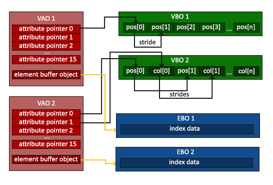
The image is taken from this tutorial .

As with buffers, vertex arrays are best viewed using their configuration example.

  unsigned int VBO, VAO; glGenBuffers(1, &VBO); glGenBuffers(1, &EBO); glGenVertexArrays(1, &VAO); glBindVertexArray(VAO); //    glBindBuffer(GL_ARRAY_BUFFER, VBO); glBufferData(GL_ARRAY_BUFFER, sizeof(vertices), vertices, GL_STATIC_DRAW); //     () glEnableVertexAttribArray(0); glVertexAttribPointer(0, 3, GL_FLOAT, GL_FALSE, 6 * sizeof(float), nullptr); //     () glEnableVertexAttribArray(1); glVertexAttribPointer(1, 3, GL_FLOAT, GL_FALSE, 6 * sizeof(float), reinterpret_cast<void*> (sizeof(float) * 3)); glBindBuffer(GL_ARRAY_BUFFER, 0); glBindVertexArray(0);
      
      

        
        
        
      

    
        
        
        
      
      

        
        
        
      

    
     

Creating vertex arrays is no different from creating other OpenGL objects, the most interesting begins after the line:

 glBindVertexArray(VAO);
      
      

        
        
        
      

    
        
        
        
      
      

        
        
        
      

    
     

  glBindBuffer(GL_ARRAY_BUFFER, VBO); glEnableVertexAttribArray(0); glVertexAttribPointer(0, 3, GL_FLOAT, GL_FALSE, 6 * sizeof(float), nullptr);
      
      

        
        
        
      

    
        
        
        
      
      

        
        
        
      

    
     

1. The attribute number that we want to configure.
2. The number of items we want to take. (Since the input variable of the vertex shader with layout = 0 is of type vec3, then we take 3 elements of type float)
3. Type of items.
4. Is it necessary to normalize the elements, if it is a vector.
5. The offset for the next vertex (since we have the coordinates and colors sequentially located and each is of type vec3, then we shift by 6 * sizeof (float) = 24 bytes).
6. The last argument shows what offset to take for the first vertex. (for coordinates, this argument is 0 bytes, for colors 12 bytes)

All now we are ready to render our first image

Remember to bind the VAO and the shader program before invoking the draw.

 { // your render loop glUseProgram(shaderProgram); glBindVertexArray(VAO); glDrawElements(GL_TRIANGLES,0,3); //        }
      
      

        
        
        
      

    
        
        
        
      
      

        
        
        
      

    
     

If you did everything right, then you should get this result:

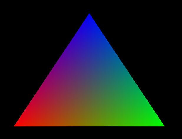
The result is impressive, but where did the gradient fill come from in the triangle, because we indicated only 3 colors: red, blue and green for each individual vertex? This is the magic of the rasterization shader: the fact is that the Color value that we set in the vertex is not getting into the fragment shader. We transfer only 3 vertices, but much more fragments are generated (there are exactly as many fragments as there are filled pixels). Therefore, for each fragment, the average of the three Color values ​​is taken, depending on how close it is to each of the vertices. This is very well seen at the corners of the triangle, where the fragments take the color value that we indicated in the vertex data.

Looking ahead, I’ll say that the texture coordinates are transmitted in the same way, which makes it easy to overlay textures on our primitives.

I think this is worth finishing this article, the most difficult is behind us, but the most interesting is just beginning. If you have questions or you saw a mistake in the article, write about it in the comments, I will be very grateful.

In the next article, we will look at transformations, learn about unifrom variables, and learn how to apply textures to primitives.