Pascal's triangle vs chains of the type “000 ... / 111 ...” in binary rows and neural networks

Series “White noise draws a black square”

The history of the cycle of these publications begins with the fact that in G.Sekey’s book “Paradoxes in Probability and Mathematical Statistics” ( p. 43 ), the following statement was discovered:





Fig. one.



According to the analysis, the commentary on the first publications ( part 1 , part 2 ) and subsequent reasoning ripened the idea to present this theorem in a more visual form.



Most of the community members are familiar with the Pascal triangle, as a consequence of the binomial probability distribution and many related laws. To understand the mechanism of the formation of Pascal's triangle, we will expand it in more detail, with the deployment of the flows of its formation. In the Pascal triangle, nodes are formed by the ratio of 0 and 1, the figure below.





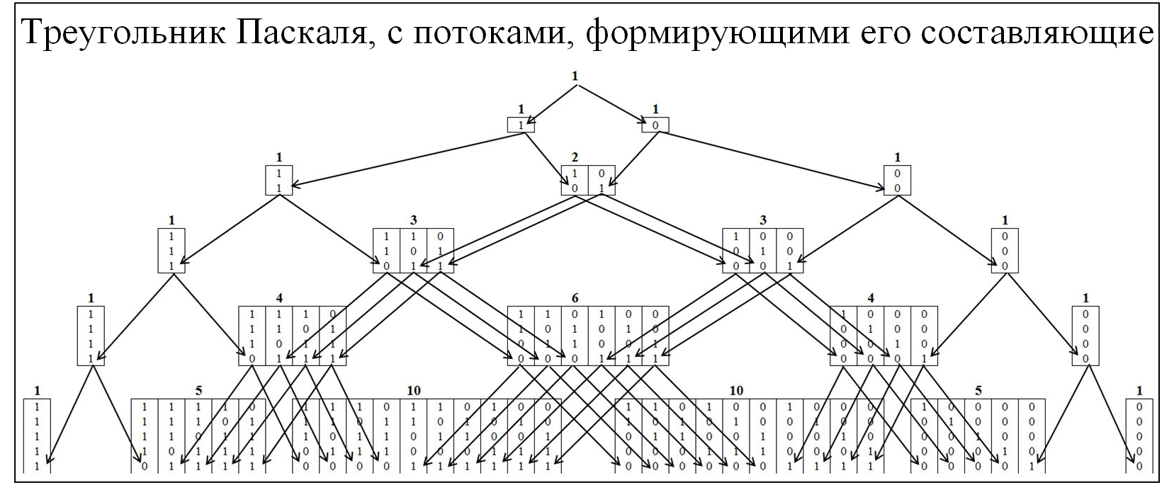
Fig. 2.



To understand the Erds-Renyi theorem, we will compose a similar model, but the nodes will be formed from the values ​​in which the largest chains are present, consisting sequentially of the same values. Clustering will be carried out according to the following rule: chains 01/10, to cluster “1”; chain 00/11, to cluster “2”; chains 000/111, to cluster "3", etc. In this case, we will break the pyramid into two symmetrical components Figure 3.





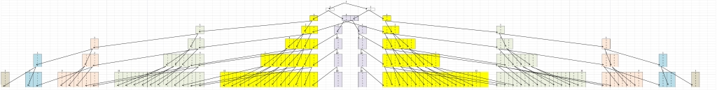
Fig. 3.



The first thing that catches your eye is that all movements occur from a lower cluster to a higher one and vice versa cannot be. This is natural, since if a chain of size j has formed, then it can no longer disappear.



By defining the algorithm for concentration of numbers, it was possible to obtain the following recurrence formula, the mechanism of which is shown in Figures 4-6.



Let us denote the elements in which the numbers are concentrated. Where n is the number of characters in the number (number of bits), and the length of the maximum chain is m. And each element will receive an index n; mJ.

Denote that the number of elements passed from n; mJ to n + 1; m + 1J, n; mjn + 1; m + 1.





Fig. four.



Figure 4 shows that for the first cluster it is not difficult to determine the values ​​of each row. And this dependence is equal to:





Fig. 5.



We determine for the second cluster, with the chain length m = 2, Figure 6.





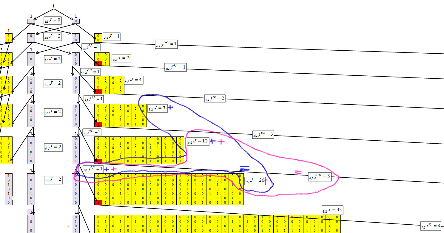
Fig. 6.



Figure 6 shows that for the second cluster, the dependence is equal to:





Fig. 7.



We determine for the third cluster, with the chain length m = 3, Figure 8.





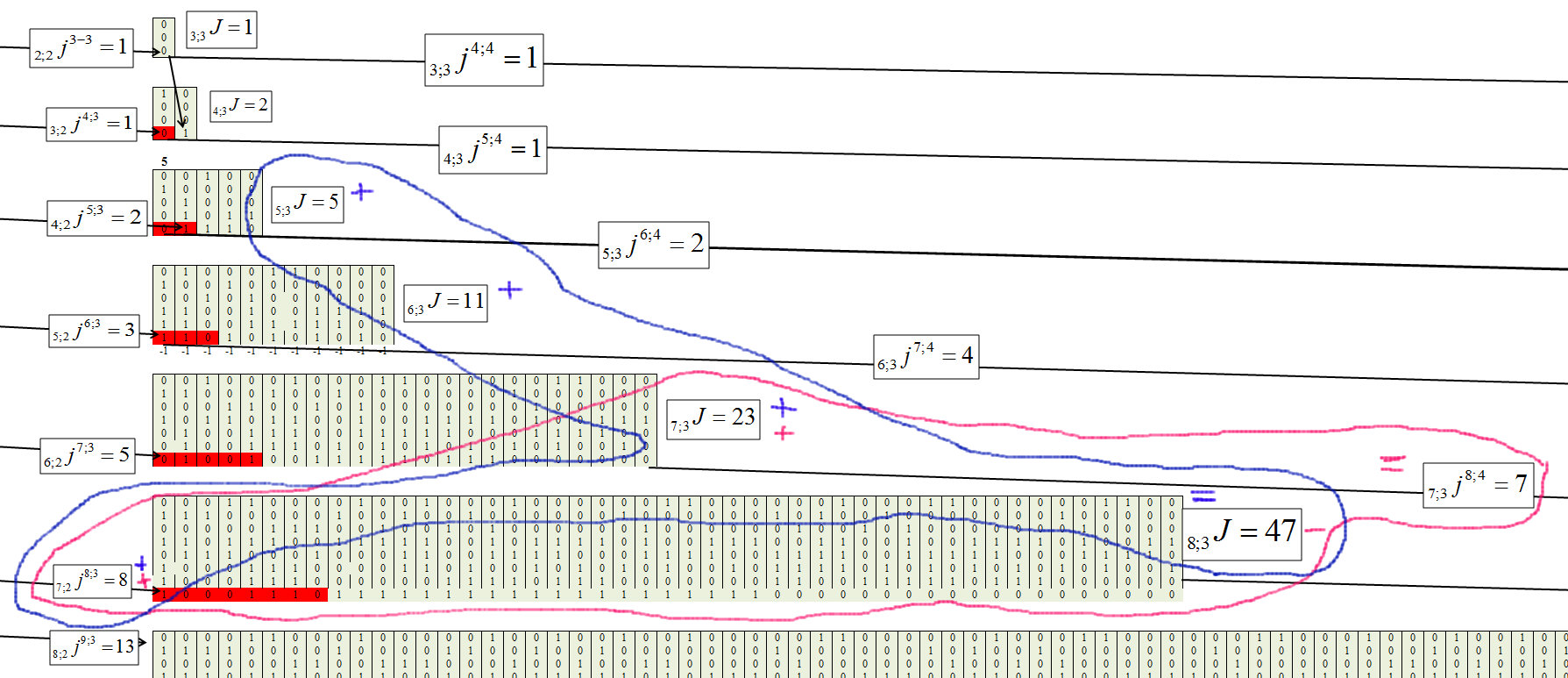
Fig. 8.



Fig. 9.



The general formula of each element takes the form:





Fig. 10.





Fig. eleven.



Verification



For verification, we use the property of this sequence, which is shown in Figure 12. It consists in the fact that the last members of a line from a certain position take a single value for all lines with increasing line length.





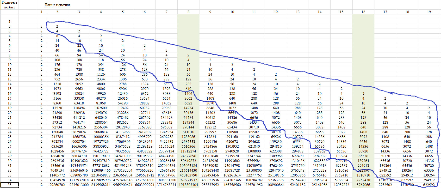
Fig. 12.



This property is due to the fact that with a chain length of more than half of the entire row, only one such chain is possible. We show this in the diagram of Figure 13.





Fig. 13.



Accordingly, for values ​​of k <n-2, we obtain the formula:





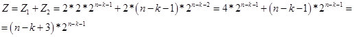
Fig. fourteen.



In fact, the Z value is the potential number of numbers (options in a string of n bits) that contain a chain of k identical elements. And according to the recurrence formula, we determine the number of numbers (options in a string of n bits) in which the chain of k identical elements is the largest. So far, I assume that the value Z is virtual. Therefore, in the region n / 2, it passes into real space. In Figure 15, a screen with calculations.





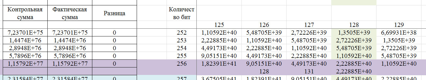
Fig. fifteen.



Let us show an example of a 256-bit word, which can be determined by this algorithm.





Fig. 16.



If determined by the standards of 99.9% reliability for the GSPCH, then the 256-bit key must contain consecutive chains of identical characters with the number from 5 to 17. That is, according to the standards for the GSPCH, so that it meets the requirement of similarity of randomness with 99.9% reliability, GSPCH, in 2000 tests (issuing a result in the form of a 256-bit binary number) should only give a result in which the maximum series length of the same values: either less than 4, or more than 17.





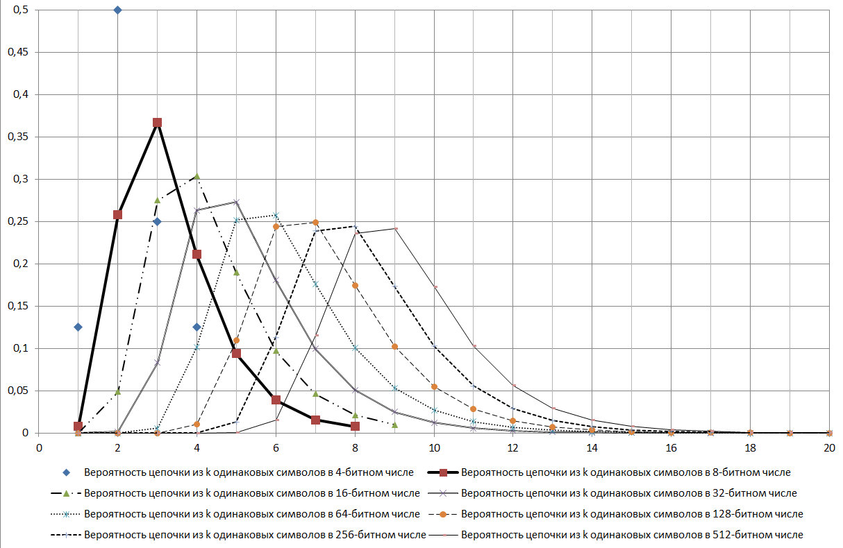
Fig. 17.



As can be seen from the diagram presented in Figure 17, the log2N chain is a mode for the distribution under consideration.



During the study, many signs of various properties of this sequence were found. Here are some of them:

• it should be well tested by the chi-square criterion;
• gives signs of the existence of fractal properties;
• may be good criteria for identifying various random processes.

And many more other connections.



Checked whether such a sequence exists on the T he On-Line Encyclopedia of Integer Sequences (OEIS) (Online Encyclopedia of Integer Sequences) in the sequence number A006980 , reference is made to the publication JL Yucas, Counting special sets of binary Lyndon words, Ars Combin. , 31 (1991), p. 21-29 , where the sequence is shown on page 28 (in the table). In the publication, the lines are numbered 1 less, but the values ​​are the same. In general, the publication about Lyndon 's words , that is, it is quite possible that the researcher did not even suspect that this series was related to this aspect.



Let us return to the Erdos-Renyi theorem. According to the results of this publication, it can be said that in the formulation that is presented, this theorem refers to the general case, which is determined by the Muavre-Laplace theorem. And the indicated theorem, in this formulation, cannot be an unambiguous criterion for the randomness of a series. But fractality, and for this case it is expressed that chains of a specified length can be combined with chains of a longer length, do not allow one to so unambiguously reject this theorem, since an inaccuracy in the formulation is possible. An example is the fact that if for 256-bit the probability of a number where the maximum chain of 8 bits is 0.244235, then, in conjunction with the other, longer sequences, the probability that a number of 8 bits is present in the number is already - 0.490234375. That is, so far, there is no unequivocal opportunity to reject this theorem. But this theorem fits quite well in another aspect, which will be shown later.



Practical use



Let's look at the example presented by the VDG user: “... The dendritic branches of a neuron can be represented as a bit sequence. A branch, and then the entire neuron, is triggered when a chain of synapses is activated in any of its places. The neuron has the task of not responding to white noise, respectively, the minimum length of the chain, as far as I remember at Numenta, is 14 synapses for the pyramidal neuron with its 10 thousand synapses. And according to the formula we get: Log_ {2} 10000 = 13.287. That is, chains less than 14 in length will occur due to natural noise, but will not activate the neuron. It’s perfectly laid right . ”



We will construct a graph, but taking into account the fact that Excel does not count values ​​greater than 2 ^ 1024, we will limit ourselves to the number of synapses 1023 and, taking this into account, we will interpolate the result by comment, as shown in Figure 18.





Fig. eighteen.



There is a biological neural network that triggers when a chain of m = log2N = 11 is compiled. This chain is a modal value, and a threshold value, probability, of some kind of change in the situation of 0.78 is reached. And the probability of error is 1- 0.78 = 0.22. Suppose a chain of 9 sensors worked, where the probability of determining the event is 0.37, respectively, the probability of error is 1 - 0.37 = 0.63. That is, in order to reduce the probability of error from 0.63 to 0.37, it is necessary that 3.33 chains of 9 elements work. The difference between 11 and 9 elements is of the 2nd order, that is 2 ^ 2 = 4 times, which if rounded to integers, since the elements give an integer value, then 3.33 = 4. We look further to reduce the error when processing a signal from 8- elements, we already need 11 triggering chains of 8 elements. I suppose that this is a mechanism that allows you to assess the situation and make a decision about changing the behavior of a biological object. Reasonably and efficiently enough, in my opinion. And taking into account the fact that we know about nature that it uses resources as economically as possible, the hypothesis that the biological system uses this mechanism is justified. And when we train the neural network, we, in fact, reduce the likelihood of error, since in order to completely eliminate the error we need to find an analytical relationship.



We turn to the analysis of numerical data. When analyzing numerical data, we try to select an analytical dependence in the form y = f (xi). And at the first stage we find it. After finding it, the existing series can be represented as binary, relative to the regression equation, where we assign 1 to positive values ​​and 0 to negative ones. And then we analyze on a series of identical elements. We determine the largest, along the length of the chain, distribution of shorter chains.



Next, we turn to the Erdos-Renyi theorem, it follows from it that when conducting a large number of tests of a random value, a chain of identical elements must be formed in all the registers of the generated number, that is, m = log2N. Now, when we examine the data, we do not know what the volume of the series really is. But if you look back, then this maximum chain gives us reason to assume that R is a parameter characterizing a field of a random variable, Figure 19.





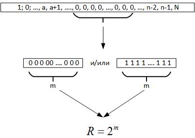
Fig. 19.



That is, comparing R and N, we can draw several conclusions:

1. If R <N, then the random process is repeated several times on historical data.
2. If R> N, then the random process has a dimension higher than the available data, or we incorrectly determined the equation of the objective function.

Then for the first case we are designing a neural network with 2 ^ m sensors, I suggest that we can add a pair of sensors to catch the transitions, and we train this network on historical data. If the network as a result of training is not able to learn and will produce the correct result with a probability of 50%, then this means that the found objective function is optimal and it is impossible to improve it. If the network can learn, then we will further improve the analytical dependence.



If the dimension of the series is greater than the dimension of a random variable, then we can use the fractal property of a random variable, since any series of size m contains all the subspaces of lower dimensions. I suppose that in this case it makes sense to train the neural network on all data except chains m.



Another approach to the design of neural networks may be the forecast period.



In conclusion, it must be said that on the way to this publication, many aspects were discovered where the dimension of a random variable and its properties were intersected with other tasks in the analysis of the data. But for now this is all in a very raw form and will be left for future publications.



Previous Part: Part 1 , Part 2