Calculation of the null hypothesis, for example, the analysis of salaries of Ukrainian programmers
I decided to share, but I myself would not forget how you can use simple statistical tools for data analysis. An anonymous survey was used as an example regarding salaries, length of service and positions of Ukrainian programmers for 2014 and 2019. (one)
After some manipulations (the code is here ), we present the data in the following form:
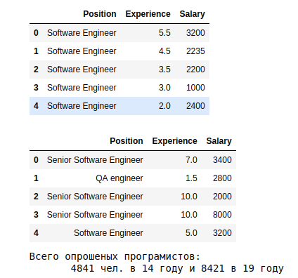
A little more groupings for one year (let the 19th):

The first estimates are as follows.
but. The results show that on average in 19, those who have been working for more than 10 years receive more than 3.5k. The dependence of experience -> zp
at. Average s.p. in 19, depending on the specialization, they show a spread of 10 times - from 5k for System Architect, to 575 for Junior QA.
from. The last plate shows the distribution by profession. Most data about Software Engineer, without qualification.
We draw attention to the features of the 19th year: Something is wrong with the 9th year of experience and there is no classification according to the levels of junior, middle, senior. You can better understand the reasons for the outlier of the 9th year. But for this analysis, we take it as it is.
But with the categories - it's worth sorting out. in 19, the Software Engineer 2739 people (35% of all) without indicating the level of qualification. Let's calculate the average and deviations for those who indicated.
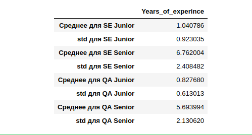
It turns out that the average work experience (who indicated it) for SE Junior is a year, with a fairly wide deviation of one year. SE Senior has the most experience with a similarly large 2.4-year deviation.
If we try to calculate Middle and use the average experience of those who indicated it, then to categorize the one who did not indicate it, we may not correctly cluster the entire sample. We will especially be mistaken in other specialties (not SE and QA) i.e. too little data. Moreover, there are few of them for comparison with the 14th year.
What else can I use?
Let's take only the salary level as a reliable indicator of the skill level! (I think there will be dissent).
First, we build what the distribution of salaries for the 19th year looks like.
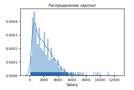
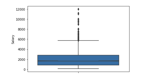
Outliers significant number after 6 $ k. We leave the range of limitations [400 - 4000]. Any programmer should get more than 400 :)
Already a little closer to the normal distribution.
We compose for 19 years, skill levels depending on the RFP. $ 3600 Range gives us a good divider into 3 categories - $ 1200
We draw - the distribution density by category for 19 years.

By adding the specified amount of experience (left corner), you can see different nuances. For example, that on average Junior gets up to 1k and his work experience is 5 years. Senior has the largest scatter in sn (a black short line at the top of each column) and many other interesting details.
This is where the first two stages are finished, we proceed to the test of hypotheses using bootstraping.
At the first stages, we found out that the specified work experience does not very accurately mean the level of qualification. Then we form the null hypothesis (the one that needs to be refuted)
There are many options (for example):
However, since the indicated experience is a bad indicator, and the calculation for certain categories can be confusing, then we take a simple and more substantive option: The average level of sn at 14, the same as in 19, is our null hypothesis H0 (2).
That is, we assume that the salaries for 5 years have not changed.
NOT the fidelity of the hypothesis, in spite of all its obviousness, we can accurately check by calculating the P-value for the null hypothesis.
The average salary in the year 14 is $ 1797, where the confidence interval is 95% [300.0 4000.0]
The average salary in 19 is $ 1949, where the confidence interval is 95% [300.0 5000.0]
The difference in average salaries in the years 14 and 19: $ 152
It is logical to choose the average values as our metric. Other options are possible, for example the median, which is often done in case of a significant number of outliers. However, the average as an estimate is easy to understand and also gives a good idea.
Writing a bootstrapping function.
We calculate our statistics.
p-value = 0.0
P-values up to 0.05 are considered insignificant, and in our case it is equal to 0. Which means the null hypothesis is disproved - the average salary in the year 14 and 19 is different and this is not an accidental result or a significant number of outliers.
We generated 10 thousand of such arrays, on average, could not get a total of more such detachments than the data themselves.
Although we spent a lot of attention on the first two stages, we formulated the correct hypothesis and chose the right metric. In more complex tasks, with a large number of variables, without such preliminary steps, analytics can lead to an incorrect interpretation. Do not skip them.
As a result of our study of the level of salaries for 14 and 19 years, we came to the following conclusions:
Thank you for your attention. I will be glad to comments and criticism.
Analysis steps
- Data preprocessing and preliminary analysis ( anyone interested in the code here )
- A graphical representation of the data. Distribution density function.
- We formulate the null hypothesis (H0) (2)
- Choosing a metric for analysis
- We use the bootstraping method to form a new data array.
- We calculate p-value (3) to confirm or refute the hypothesis
Data preprocessing
After some manipulations (the code is here ), we present the data in the following form:
# , . display(data_14_1.head(), data_19_1.head()) print(' : \n \ {} . 14 {} 19 '.format(len(data_14_1), len(data_19_1)))
A little more groupings for one year (let the 19th):
# , 19 display(pd.DataFrame(df.groupby(['Experience'])['Salary'].mean().sort_values(ascending=False)), \ pd.DataFrame(df.groupby(['Position'])['Salary'].mean().sort_values(ascending=False)), \ df.Position.value_counts())
The first estimates are as follows.
but. The results show that on average in 19, those who have been working for more than 10 years receive more than 3.5k. The dependence of experience -> zp
at. Average s.p. in 19, depending on the specialization, they show a spread of 10 times - from 5k for System Architect, to 575 for Junior QA.
from. The last plate shows the distribution by profession. Most data about Software Engineer, without qualification.
We draw attention to the features of the 19th year: Something is wrong with the 9th year of experience and there is no classification according to the levels of junior, middle, senior. You can better understand the reasons for the outlier of the 9th year. But for this analysis, we take it as it is.
But with the categories - it's worth sorting out. in 19, the Software Engineer 2739 people (35% of all) without indicating the level of qualification. Let's calculate the average and deviations for those who indicated.
It turns out that the average work experience (who indicated it) for SE Junior is a year, with a fairly wide deviation of one year. SE Senior has the most experience with a similarly large 2.4-year deviation.
If we try to calculate Middle and use the average experience of those who indicated it, then to categorize the one who did not indicate it, we may not correctly cluster the entire sample. We will especially be mistaken in other specialties (not SE and QA) i.e. too little data. Moreover, there are few of them for comparison with the 14th year.
What else can I use?
Let's take only the salary level as a reliable indicator of the skill level! (I think there will be dissent).
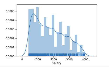
First, we build what the distribution of salaries for the 19th year looks like.
Outliers significant number after 6 $ k. We leave the range of limitations [400 - 4000]. Any programmer should get more than 400 :)
df_new = data_19_1[(data_19_1['Salary'] > 400) & (data_19_1['Salary'] < 4000)] sns.distplot(df_new['Salary'], rug=True, norm_hist=True)
Already a little closer to the normal distribution.
We compose for 19 years, skill levels depending on the RFP. $ 3600 Range gives us a good divider into 3 categories - $ 1200
df_new.reset_index() df_new.loc['level'] = 0 df_new.loc[df_new.Salary <= 1200, 'level'] = 'Junior' df_new.loc[(df_new.Salary > 1200) & (df_new.Salary <= 2400), 'level'] = 'Middle' df_new.loc[df_new.Salary > 2401, 'level'] = 'Senior'
We draw - the distribution density by category for 19 years.
sns.set(style="whitegrid") fig, ax = plt.subplots() fig.set_size_inches(11.7, 8.27) plt.title(' 19 ') sns.barplot(x='level', y='Salary', hue='Experience', hue_order=[1,3,5,7,10], palette='Blues', \ data=df_new, ci='sd')
By adding the specified amount of experience (left corner), you can see different nuances. For example, that on average Junior gets up to 1k and his work experience is 5 years. Senior has the largest scatter in sn (a black short line at the top of each column) and many other interesting details.
This is where the first two stages are finished, we proceed to the test of hypotheses using bootstraping.
We formulate the null hypothesis (H0)
At the first stages, we found out that the specified work experience does not very accurately mean the level of qualification. Then we form the null hypothesis (the one that needs to be refuted)
There are many options (for example):
- The dependence of salary on seniority in the year 14 is the same as in the 19th.
- Junior salaries have not changed since 14 years.
However, since the indicated experience is a bad indicator, and the calculation for certain categories can be confusing, then we take a simple and more substantive option: The average level of sn at 14, the same as in 19, is our null hypothesis H0 (2).
That is, we assume that the salaries for 5 years have not changed.
NOT the fidelity of the hypothesis, in spite of all its obviousness, we can accurately check by calculating the P-value for the null hypothesis.
# (14 19 ), 95 % mean_salary_14 = np.mean(data_14_1['Salary']) conf_salary_14 = np.percentile(data_14_1['Salary'], [2.5, 97.5]) mean_salary_19 = np.mean(data_19_1['Salary']) conf_salary_19 = np.percentile(data_19_1['Salary'], [2.5, 97.5]) diff_mean_salary = mean_salary_19 - mean_salary_14
The average salary in the year 14 is $ 1797, where the confidence interval is 95% [300.0 4000.0]
The average salary in 19 is $ 1949, where the confidence interval is 95% [300.0 5000.0]
The difference in average salaries in the years 14 and 19: $ 152
Metric for analysis
It is logical to choose the average values as our metric. Other options are possible, for example the median, which is often done in case of a significant number of outliers. However, the average as an estimate is easy to understand and also gives a good idea.
Writing a bootstrapping function.
# bootstraping def bootstrap(data, func): boots = np.random.choice(data, len(data)) return func(boots) def bootstrapping(data, func=np.mean, size=1): reps = np.empty(size) for i in range(size): reps[i] = bootstrap(data, func) return reps
We calculate our statistics.
# 14 19 - data = np.concatenate((data_14_1['Salary'].values, data_19_1['Salary'].values)) # 2 data_mean = np.mean(data) # 14 19 , data_14_shifted = data_14_1['Salary'].values - np.mean(data_14_1['Salary'].values) + data_mean data_19_shifted = data_19_1['Salary'].values - np.mean(data_19_1['Salary'].values) + data_mean # 10000 , data_14_bootsted = bootstrapping(data_14_shifted, np.mean, size=10000) data_19_bootsted = bootstrapping(data_19_shifted, np.mean, size=10000) # . . mean_diff = data_19_bootsted - data_14_bootsted # P value . p_value = sum(mean_diff >= diff_mean_salary) / len(mean_diff) print('p-value = {}'.format(p_value))
p-value = 0.0
P-values up to 0.05 are considered insignificant, and in our case it is equal to 0. Which means the null hypothesis is disproved - the average salary in the year 14 and 19 is different and this is not an accidental result or a significant number of outliers.
We generated 10 thousand of such arrays, on average, could not get a total of more such detachments than the data themselves.
Although we spent a lot of attention on the first two stages, we formulated the correct hypothesis and chose the right metric. In more complex tasks, with a large number of variables, without such preliminary steps, analytics can lead to an incorrect interpretation. Do not skip them.
As a result of our study of the level of salaries for 14 and 19 years, we came to the following conclusions:
- Based on the survey data, the specified length of service is not an entirely suitable criterion for determining the level of salaries and qualifications.
- The division into the skill level will most likely be based on the level of salaries.
- The salaries of programmers increased from 14 to 19 (an average of 8.5%) and this is not an accidental result.
Thank you for your attention. I will be glad to comments and criticism.
Sources
All Articles