Face Recognition Using Siamese Networks

Siamese neural network is one of the simplest and most popular single-learning algorithms. Methods in which for each class is taken only one case study. Thus, the Siamese network is usually used in applications where there are not many units of data in each class.



Suppose we need to make a face recognition model for an organization that employs about 500 people. If you make such a model from scratch based on the convolutional neural network (CNN), then to train the model and achieve good recognition accuracy, we will need many images of each of these 500 people. But it’s obvious that we cannot compile such a dataset, so you should not make a model based on CNN or any other deep learning algorithm if we don’t have enough data. In such cases, you can use the complex one-time learning algorithm, like the Siamese network, which can be trained on less data.



In fact, Siamese networks consist of two symmetric neural networks, with the same weights and architecture, which at the end combine and use the energy function - E.

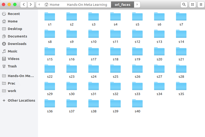
Let's look at the Siamese network, creating a face recognition model on its basis. We will teach her to determine when two faces are the same and when not. And for starters, we’ll use the AT&T Database of Faces dataset, which can be downloaded from the Cambridge University computer lab website.



Download, unpack and see folders from s1 to s40:







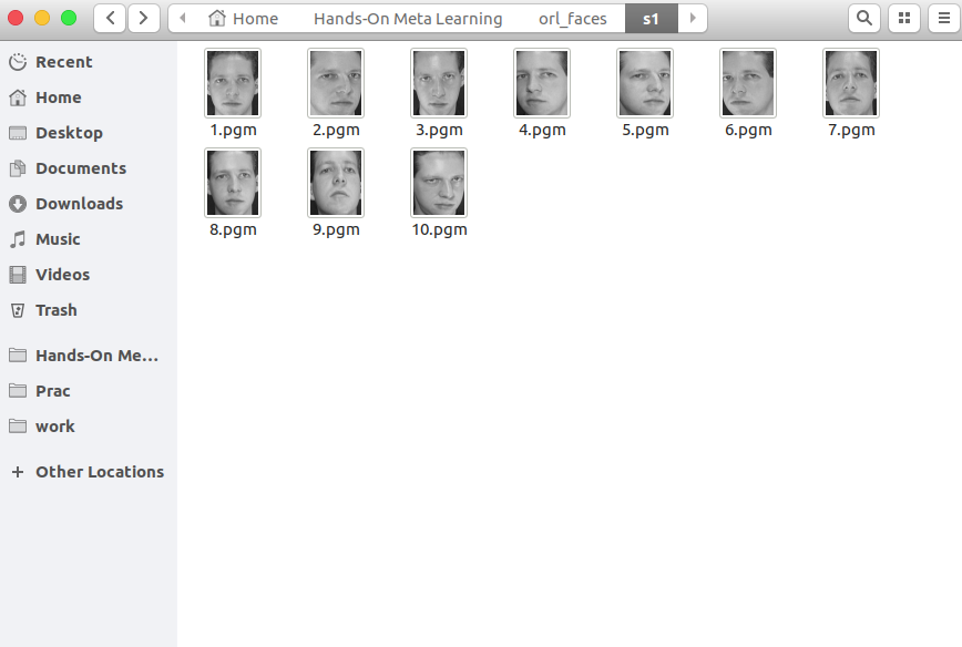
Each folder contains 10 different photographs of a single person taken from different angles. Here is the contents of the s1 folder:







And here’s what’s in the s13 folder:







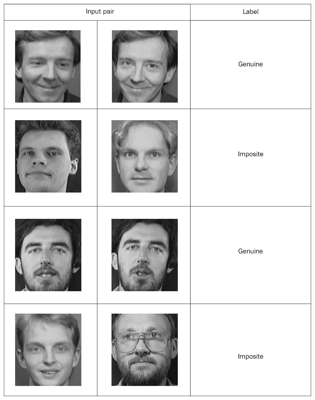
Siamese networks need to input paired values ​​with markings, so let's create such sets. Take two random photos from the same folder and mark them as a “genuine” pair. Then we take two photos from different folders and mark them as a “false” pair (imposite):







Having distributed all the photos into marked pairs, we will study the network. From each pair, we will transfer one photo to network A, and the second to network B. Both networks only extract property vectors. To do this, we use two convolutional layers with the activation of rectified linear unit (ReLU). Having studied the properties, we transfer the vectors generated by both networks into an energy function that estimates the similarity. We use the Euclidean distance as a function.

Now consider all these steps in more detail.

First, import the necessary libraries:

import re import numpy as np from PIL import Image from sklearn.model_selection import train_test_split from keras import backend as K from keras.layers import Activation from keras.layers import Input, Lambda, Dense, Dropout, Convolution2D, MaxPooling2D, Flatten from keras.models import Sequential, Model from keras.optimizers import RMSprop
      
      

        
        
        
      

    
        
        
        
      
      

        
        
        
      

    
     

Now we define a function for reading input images. The read_image



function takes a picture and returns a NumPy array:

 def read_image(filename, byteorder='>'): #first we read the image, as a raw file to the buffer with open(filename, 'rb') as f: buffer = f.read() #using regex, we extract the header, width, height and maxval of the image header, width, height, maxval = re.search( b"(^P5\s(?:\s*#.*[\r\n])*" b"(\d+)\s(?:\s*#.*[\r\n])*" b"(\d+)\s(?:\s*#.*[\r\n])*" b"(\d+)\s(?:\s*#.*[\r\n]\s)*)", buffer).groups() #then we convert the image to numpy array using np.frombuffer which interprets buffer as one dimensional array return np.frombuffer(buffer, dtype='u1' if int(maxval)
      
      

        
        
        
      

    
        
        
        
      
      

        
        
        
      

    
     

For example, open this photo:

 Image.open("data/orl_faces/s1/1.pgm")
      
      

        
        
        
      

    
        
        
        
      
      

        
        
        
      

    
     

We pass it to the read_image



function and get a NumPy array:

 img = read_image('data/orl_faces/s1/1.pgm') img.shape (112, 92)
      
      

        
        
        
      

    
        
        
        
      
      

        
        
        
      

    
     

Now we define the get_data



function that will generate the data. Let me remind you that Siamese networks need to submit data pairs (genuine and imposite) with binary marking.



First, read the images ( img1



, img2



) from one directory, save them in the x_genuine_pair,



array x_genuine_pair,



set y_genuine



to 1



. Then read the images ( img1



, img2



) from different directories, save them in the x_imposite,



pair x_imposite,



and set y_imposite



to 0



.



Concatenate x_genuine_pair



and x_imposite



in X



, and y_genuine



and y_imposite



in Y



:

 size = 2 total_sample_size = 10000 def get_data(size, total_sample_size): #read the image image = read_image('data/orl_faces/s' + str(1) + '/' + str(1) + '.pgm', 'rw+') #reduce the size image = image[::size, ::size] #get the new size dim1 = image.shape[0] dim2 = image.shape[1] count = 0 #initialize the numpy array with the shape of [total_sample, no_of_pairs, dim1, dim2] x_geuine_pair = np.zeros([total_sample_size, 2, 1, dim1, dim2]) # 2 is for pairs y_genuine = np.zeros([total_sample_size, 1]) for i in range(40): for j in range(int(total_sample_size/40)): ind1 = 0 ind2 = 0 #read images from same directory (genuine pair) while ind1 == ind2: ind1 = np.random.randint(10) ind2 = np.random.randint(10) # read the two images img1 = read_image('data/orl_faces/s' + str(i+1) + '/' + str(ind1 + 1) + '.pgm', 'rw+') img2 = read_image('data/orl_faces/s' + str(i+1) + '/' + str(ind2 + 1) + '.pgm', 'rw+') #reduce the size img1 = img1[::size, ::size] img2 = img2[::size, ::size] #store the images to the initialized numpy array x_geuine_pair[count, 0, 0, :, :] = img1 x_geuine_pair[count, 1, 0, :, :] = img2 #as we are drawing images from the same directory we assign label as 1. (genuine pair) y_genuine[count] = 1 count += 1 count = 0 x_imposite_pair = np.zeros([total_sample_size, 2, 1, dim1, dim2]) y_imposite = np.zeros([total_sample_size, 1]) for i in range(int(total_sample_size/10)): for j in range(10): #read images from different directory (imposite pair) while True: ind1 = np.random.randint(40) ind2 = np.random.randint(40) if ind1 != ind2: break img1 = read_image('data/orl_faces/s' + str(ind1+1) + '/' + str(j + 1) + '.pgm', 'rw+') img2 = read_image('data/orl_faces/s' + str(ind2+1) + '/' + str(j + 1) + '.pgm', 'rw+') img1 = img1[::size, ::size] img2 = img2[::size, ::size] x_imposite_pair[count, 0, 0, :, :] = img1 x_imposite_pair[count, 1, 0, :, :] = img2 #as we are drawing images from the different directory we assign label as 0. (imposite pair) y_imposite[count] = 0 count += 1 #now, concatenate, genuine pairs and imposite pair to get the whole data X = np.concatenate([x_geuine_pair, x_imposite_pair], axis=0)/255 Y = np.concatenate([y_genuine, y_imposite], axis=0) return X, Y
      
      

        
        
        
      

    
        
        
        
      
      

        
        
        
      

    
     

Now we will generate the data and check their size. We have 20,000 photos, of which 10,000 genuine and 10,000 false pairs were collected:

 X, Y = get_data(size, total_sample_size) X.shape (20000, 2, 1, 56, 46) Y.shape (20000, 1)
      
      

        
        
        
      

    
        
        
        
      
      

        
        
        
      

    
     

We will share the entire array of information: 75% of the pairs will go to training, and 25% - to testing:

x_train, x_test, y_train, y_test = train_test_split(X, Y, test_size=.25)







Now create a Siamese network. First we define the core network - it will be a convolutional neural network to extract properties. We will create two convolutional layers using ReLU activations and a layer with determination of the maximum value (max pooling) after the flat layer:

 def build_base_network(input_shape): seq = Sequential() nb_filter = [6, 12] kernel_size = 3 #convolutional layer 1 seq.add(Convolution2D(nb_filter[0], kernel_size, kernel_size, input_shape=input_shape, border_mode='valid', dim_ordering='th')) seq.add(Activation('relu')) seq.add(MaxPooling2D(pool_size=(2, 2))) seq.add(Dropout(.25)) #convolutional layer 2 seq.add(Convolution2D(nb_filter[1], kernel_size, kernel_size, border_mode='valid', dim_ordering='th')) seq.add(Activation('relu')) seq.add(MaxPooling2D(pool_size=(2, 2), dim_ordering='th')) seq.add(Dropout(.25)) #flatten seq.add(Flatten()) seq.add(Dense(128, activation='relu')) seq.add(Dropout(0.1)) seq.add(Dense(50, activation='relu')) return seq
      
      

        
        
        
      

    
        
        
        
      
      

        
        
        
      

    
     

Then we will transfer a pair of images of the core network, which will return vector representations, that is, property vectors:

 input_dim = x_train.shape[2:] img_a = Input(shape=input_dim) img_b = Input(shape=input_dim) base_network = build_base_network(input_dim) feat_vecs_a = base_network(img_a) feat_vecs_b = base_network(img_b)
      
      

        
        
        
      

    
        
        
        
      
      

        
        
        
      

    
     

feat_vecs_a



and feat_vecs_b



are property vectors of a pair of images. Let's pass their energy functions to calculate the distance between them. And as a function of energy, we use the Euclidean distance:

 def euclidean_distance(vects): x, y = vects return K.sqrt(K.sum(K.square(x - y), axis=1, keepdims=True)) def eucl_dist_output_shape(shapes): shape1, shape2 = shapes return (shape1[0], 1) distance = Lambda(euclidean_distance, output_shape=eucl_dist_output_shape)([feat_vecs_a, feat_vecs_b])
      
      

        
        
        
      

    
        
        
        
      
      

        
        
        
      

    
     

We set the number of epochs to 13, apply the RMS property for optimization and declare the model:

 epochs = 13 rms = RMSprop() model = Model(input=[input_a, input_b], output=distance)
      
      

        
        
        
      

    
        
        
        
      
      

        
        
        
      

    
     

Now we define the loss function contrastive_loss



function and compile the model:

 def contrastive_loss(y_true, y_pred): margin = 1 return K.mean(y_true * K.square(y_pred) + (1 - y_true) * K.square(K.maximum(margin - y_pred, 0))) model.compile(loss=contrastive_loss, optimizer=rms)
      
      

        
        
        
      

    
        
        
        
      
      

        
        
        
      

    
     

Let's study the model:

 img_1 = x_train[:, 0] img_2 = x_train[:, 1] model.fit([img_1, img_2], y_train, validation_split=.25, batch_size=128, verbose=2, nb_epoch=epochs)
      
      

        
        
        
      

    
        
        
        
      
      

        
        
        
      

    
     

You see how losses decrease as eons pass:

 Train on 11250 samples, validate on 3750 samples Epoch 1/13 - 60s - loss: 0.2179 - val_loss: 0.2156 Epoch 2/13 - 53s - loss: 0.1520 - val_loss: 0.2102 Epoch 3/13 - 53s - loss: 0.1190 - val_loss: 0.1545 Epoch 4/13 - 55s - loss: 0.0959 - val_loss: 0.1705 Epoch 5/13 - 52s - loss: 0.0801 - val_loss: 0.1181 Epoch 6/13 - 52s - loss: 0.0684 - val_loss: 0.0821 Epoch 7/13 - 52s - loss: 0.0591 - val_loss: 0.0762 Epoch 8/13 - 52s - loss: 0.0526 - val_loss: 0.0655 Epoch 9/13 - 52s - loss: 0.0475 - val_loss: 0.0662 Epoch 10/13 - 52s - loss: 0.0444 - val_loss: 0.0469 Epoch 11/13 - 52s - loss: 0.0408 - val_loss: 0.0478 Epoch 12/13 - 52s - loss: 0.0381 - val_loss: 0.0498 Epoch 13/13 - 54s - loss: 0.0356 - val_loss: 0.0363
      
      

        
        
        
      

    
        
        
        
      
      

        
        
        
      

    
     

And now let's test the model on test data:

 pred = model.predict([x_test[:, 0], x_test[:, 1]])
      
      

        
        
        
      

    
        
        
        
      
      

        
        
        
      

    
     

Define a function to calculate the accuracy:

 def compute_accuracy(predictions, labels): return labels[predictions.ravel()
      
      

        
        
        
      

    
        
        
        
      
      

        
        
        
      

    
     

We calculate the accuracy:

 compute_accuracy(pred, y_test) 0.9779092702169625
      
      

        
        
        
      

    
        
        
        
      
      

        
        
        
      

    
     

findings

In this guide, we learned how to create face recognition models based on Siamese networks. The architecture of such networks consists of two identical neural networks having the same weight and structure, and the results of their work are transferred to one energy function - this determines the identity of the input data. For more information on meta-learning with Python, see Hands-On Meta-Learning with Python.

My comment

Knowledge of Siamese networks is currently required when working with images. There are many approaches to training networks in small samples, new data generation, augmentation methods. This method allows relatively “cheap” to achieve good results, here is a more classic example of the Siamese network on “Hello world” for neural networks - dataset MNIST keras.io/examples/mnist_siamese