Hilbert, Lebesgue ... and the Void

Under the cut, the question of how a good multidimensional indexing algorithm should be arranged is investigated. Surprisingly, there are not so many options.
One-Dimensional Indices, B-Trees
We will consider 2 facts as the measure of success of the search algorithm -
- the establishment of the fact of its presence or absence of a result occurs for the logarithmic (with respect to the size of the index) number of reads of disk pages
- the cost of issuing a result is proportional to its volume
In this sense, B-trees are quite successful and the reason for this can be considered the use of a balanced tree. The simplicity of the algorithm is due to the one-dimensionality of the key space - if necessary, split the page, it is enough to split in half the sorted set of elements of this page. Generally divided by the number of elements, although this is not necessary.
Because the pages of the tree are stored on disk, it can be said that the B-tree has the ability to very efficiently convert one-dimensional key space to one-dimensional disk space.
When filling a tree with more or less “right insertion”, and this is a fairly common case, pages are generated in the order of growth of the key, occasionally alternating with higher pages. There are good chances that they will be on the disk too. Thus, without any effort, a high locality of data is achieved - data of similar importance will be somewhere nearby and on disk.
Of course, when inserting values in random order, the keys and pages are generated randomly, as a result of which the so-called index fragmentation. There are also anti-fragmentation tools that restore data locality.
It would seem that in our age of RAID and SSD disks the order of reading from the disk does not matter. But, rather, it does not have the same meaning as before. There is no physical forwarding of the heads in the SSD, so its random read speed does not drop hundreds of times compared to solid reading, like an HDD. And only once every 10 or more .
Recall that B-trees appeared in 1970 in the era of magnetic tapes and drums. When the difference in random access speed for the mentioned tape and drum was much more dramatic than in comparison with HDD and SSD.
In addition, 10 times also matter. And these 10 times include not only the physical features of the SSD, but also the fundamental point - the predictability of reader behavior. If the reader is very likely to ask for the next block for this block, it makes sense to download it proactively, by assumption. And if the behavior is chaotic, all attempts at prediction are meaningless and even harmful.
Multidimensional indexing
Further we will deal with the index of two-dimensional points (X, Y), simply because it is convenient and clear to work with them. But the problems are basically the same.
A simple, “unsophisticated” option with separate indices for X and Y does not pass according to our success criterion. It does not give the logarithmic cost of obtaining the first point. In fact, to answer the question, is there anything at all in the desired extent, we must
- do a search in the index X and get all the identifiers from the X-interval extent
- similar for Y
- intersect these two sets of identifiers
The first point already depends on the size of the extent and does not guarantee the logarithm.
To be “successful,” a multidimensional index must be arranged as a more or less balanced tree. This statement may seem controversial. But the requirement of a logarithmic search dictates to us just such a device. Why not two trees or more? Already considered the "unsophisticated" and unsuitable option with two trees. Perhaps there are suitable ones. But two trees - this is twice as much (including simultaneous) locks, twice as much cost, significantly greater chances to catch a deadlock. If you can get by with one tree, you should definitely use it.
Given all this, it is quite natural to want to take as a basis a very successful B-tree experience and “generalize” it to work with two-dimensional data.
So the R-tree appeared.
R-tree
The R-tree is arranged as follows:
Initially, we have a blank page, just add data (points) to it.
But the page has overflowed and it needs to be split.
In the B-tree, the page elements are ordered in a natural way, so the question is how much to cut. There is no natural order in the R-tree. There are two options:
- Bring order, i.e. introduce a function that, based on X&Y, will give out a value according to which page elements will be ordered and divided according to it. In this case, the entire index degenerates into a regular B-tree constructed from the values of the specified function. In addition to the obvious pluses, there is a big question - well, well, we indexed, but how to look? More about this later, first consider the second option.
- Divide the page by spatial criteria. To do this, each page should be assigned the extent of the elements located on / below it. Those. the root page has the extent of the entire layer. When splitting, two (or more) pages are generated, the extents of which are included in the extent of the parent page (for search).
There is sheer uncertainty. How exactly to split the page? Horizontal or vertical? Proceed from half the area or half of the elements? But what if the points formed two clusters, but you can only separate them with a diagonal line? And if there are three clusters?
The mere presence of such questions indicates that the R-tree is not an algorithm. This is a set of heuristics, at least for splitting a page during insertion, for merging pages during deletion / modification, for preprocessing for bulk insertion.
Heuristics involves the specialization of a particular tree on a particular data type. Those. on datasets of a certain kind, she errs less often. “Heuristics cannot be completely mistaken, because in this case, it would be an algorithm ”©.
What does heuristic error mean in this context? For example, that the page will be split / merged unsuccessfully and the pages will begin to partially overlap each other. If suddenly the search extent falls on the overlapping area of the pages, the cost of the search will already be not quite logarithmic. Over time, as you insert / delete, the number of errors accumulates and the performance of the tree begins to degrade.
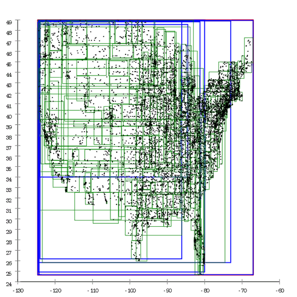
Figure 1 Here is an example of an R * tree that is built in a natural way.
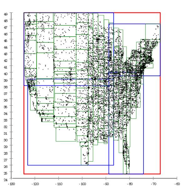
Figure 2 And here the same dataset is pre-processed and the tree is built by mass insertion
We can say that the B-tree also degrades over time, but this is a slightly different degradation. B-tree performance falls due to the fact that its pages are not in a row. This is easily treated by “straightening” the tree - defragmentation. In the case of the R-tree, it is not so easy to get rid of it; the structure of the tree itself is “curve" in order to correct the situation;
Generalizations of the R-tree to multidimensional spaces are not obvious. For example, when splitting pages, we minimized the perimeter of child pages. What to minimize in the three-dimensional case? Volume or surface area? And in the eight-dimensional case? Common sense is no longer an adviser.
Indexed space may well be non-isotropic. Why not index not just points, but their positions in time, i.e. (X, Y, t). In this case, for example, a heuristic based on the perimeter is meaningless since stacks the length at time intervals.
The general impression of the R-tree is something like gill-footed crustaceans. Those have their own ecological niche in which it is difficult to compete with them. But in the general case, they have no chance in competition with more developed animals.
Quad tree
In a quadtree, each non-leaf page has exactly four descendants, which equally divide its space into quadrants.
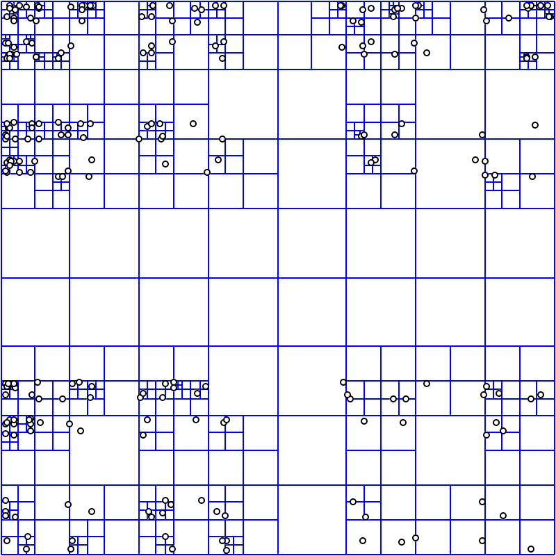
Figure 3 An example of a built quad tree
This is not a good database design.
- Each page narrows the search space for each coordinate only twice. Yes, this provides the logarithmic complexity of the search, but this is the base 2 logarithm, not the number of elements on the page, (even 100) as in the B-tree.
- Each page is small, but behind it you still have to go to disk.
- The depth of the quad tree must be limited, otherwise its imbalance affects performance. As a result, on highly clustered data (for example, houses on the map — there are a lot of cities in the cities, few in the fields) a large amount of data can accumulate on the sheet pages. An index from an exact one becomes blocky and requires post-processing.
A poorly selected grid size (tree depth) can kill performance. Nevertheless, I would like for the performance of the algorithm not to depend critically on the human factor.
- The cost of space for storing one point is quite large.
Space numbering
It remains to consider the previously deferred version with a function that, based on a multidimensional key, calculates the value for writing in a regular B-tree.
The construction of such an index is obvious, and the index itself has all the advantages of the B-tree. The only question is whether this index can be used for effective search.
There are a huge number of such functions, it can be assumed that among them there are a small number of “good”, a large number of “bad” and a huge number of “just awful”.
Finding a terrible function is not difficult - we serialize the key into a string, consider MD5 from it and get a value that is completely useless for our purposes.
And how to approach the good? It has already been said that a useful index provides “locality” of data - points that are close in space and often are close to each other when saved to disk. As applied to the desired function, this means that for spatially close points it gives close values.
Once in the index, the calculated values will appear on the "physical" pages in the order of their values. From a “physical sense” point of view, the search extent should affect as few physical index pages as possible. What is generally obvious. From this point of view, the numbering curves that “pull” the data are “bad”. And those that “confuse in a ball” - closer to the “good”.
Naive numbering
An attempt to squeeze a segment into a square (hypercube) while remaining in the logic of one-dimensional space i.e. cut into pieces and fill the square with these pieces. It could be
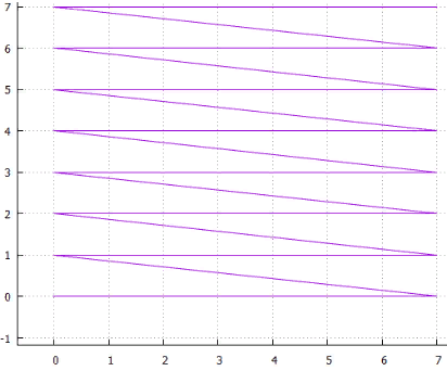
4 line scan
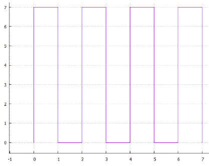
5 interlaced
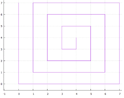
Fig.6 spiral
or ... you can come up with a lot of options, all of them have two drawbacks
- ambiguity, for example: why the spiral is curled clockwise and not against it, or why the horizontal scan is first along X and then along Y
- the presence of long straight pieces that make the use of such a method ineffective for multidimensional indexing (large page perimeter)
Direct access features
If the main claim to “naive” methods is that they generate very elongated pages, let's generate the “correct” pages on our own.
The idea is simple - let there be an external partition of space into blocks, assign an identifier to each block and this will be the key of the spatial index.
- let the X&Y coordinates be 16-bit (for clarity)
- we are going to cover the space with square blocks of size 1024X1024
- coarsen the coordinates, shift by 10 bits to the right
- and get the page identifier, glue the bits from X&Y. Now in the identifier the lower 6 digits are the oldest from X, the next 6 digits are the oldest from Y
It is easy to see that the blocks form a line scan, therefore, to find data for the search extent, you will have to do a search / read in the index for each row of blocks that this extent has laid on. In general, this method works great, although it has several disadvantages.
- when creating an index, you have to choose the optimal block size, which is completely unobvious
- if the block is significantly larger than a typical query, the search will be inefficient since have to read and filter (postprocessing) too much
- if the block is significantly smaller than a typical query, the search will be inefficient since will have to do a lot of queries row by row
- if the block has too much or too little data on average, the search will be ineffective
- if the data is clustered (ex: at home on the map), the search will not be effective everywhere
- if the dataset has grown, it may well turn out that the block size has ceased to be optimal.
Partially, these problems are solved by building multi-level blocks. For the same example:
- still want 1024X1024 blocks
- but now we will still have top-level blocks of size 8X8 lower blocks
- the key is arranged as follows (from low to high):
3 digits - digits 10 ... 12 X coordinates
3 digits - digits 10 ... 12 Y coordinates
3 digits - digits 13 ... 15 X coordinates
3 digits - digits 13 ... 15 Y coordinates
7 Low-level blocks form high-level blocks
Now for large extents you don’t need to read a huge number of small blocks, this is done at the expense of high-level blocks.
Interestingly, it was possible not to roughen the coordinates, but in the same manner to squeeze them into the key. In this case, post-filtering would be cheaper because would occur when reading the index.
Spatial GRID indexes are arranged in MS SQL in a similar way; up to 4 block levels are allowed in them.
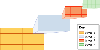
Fig.8 GRID index
Another interesting way of direct indexing is to use a quad tree for external partitioning of space.
The quad tree is useful in that it can adapt to the density of objects since when the node overflows, it splits. As a result, where the density of objects is high, the blocks will turn out small and vice versa. This reduces the number of empty index calls.
True, the quad tree is an inconvenient construction for rebuilding on the fly, it is advantageous to do this from time to time.
From the pleasant thing, when rebuilding a quad tree, there is no need to rebuild the index if the blocks are identified by the Morton code and objects are encoded using it. Here's the trick: if the coordinates of the point are encoded with a Morton code, the page identifier is a prefix in that code. When searching for page data, all keys that are in the range from [prefix] 00 ... 00B to [prefix] 11 ... 11B are selected, if the page is split, it means only the prefix of its descendants has lengthened.
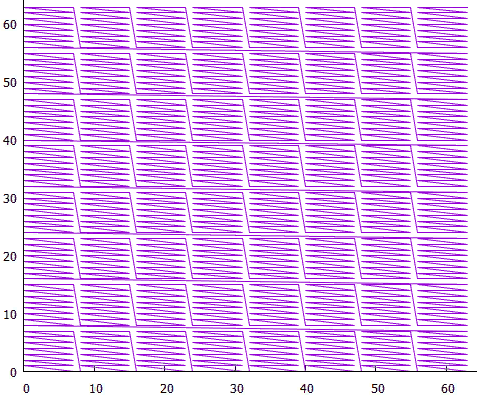
Self-similar features
The first thing that comes to mind when mentioning self-similar functions is “sweeping curves”. “A noticeable curve is a continuous mapping, the domain of which is the unit segment [0, 1], and the domain is the Euclidean (more strictly, topological) space.” An example is the Peano curve.
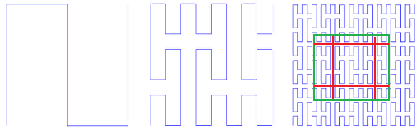
Fig. 9 first iterations of the Peano curve
In the lower left corner is the beginning of the definition area (and the function's zero value), in the upper right corner the end (and 1), each time we move 1 step, add 1 / (N * N) to the value (provided that N - degree 3, of course). As a result, in the upper right corner, the value reaches 1. If we add one at each step, such a function simply sequentially numbers the square lattice, which is what we wanted.
All sweeping curves are self-similar. In this case, the simplex is a 3x3 square. At each iteration, each point of the simplex turns into the same simplex, to ensure continuity, you have to resort to mappings (flips).
Self - similarity is a very important quality for us. It gives hope for the logarithmic value of the search. For example, for a 3x3 simplex, all numbers generated within each of 9 elementary squares by subsequent iterations of detail will be within the same range. Just because the number is the path traveled from the beginning. Those. if you divide the extent into 9 parts, the contents of each of them can be obtained by one index traverse. And so on recursively, each of the 9 sub-squares of each of the squares can be obtained by a single query on the index (though in a smaller range). So the search extent can be broken down into a small number of square subqueries, read either in whole or with filtering (around the perimeter). Figure 9 shows the search extent in green, broken by red lines into subqueries.
However, self-similarity does not automatically make the numbering curve suitable for indexing purposes.
- the curve should fill the square grid. We index the values in the nodes of the square lattice and each time we do not want to look for a suitable node on the lattice, for example, triangular. At least in order to avoid problems with rounding. Here, for example, such (Figure 10)
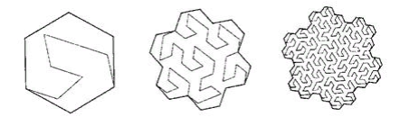
Figure 10 ternary lake Kokha
the curve does not suit us. Although, it perfectly “bridges” the surface.
- the curve should fill the space without gaps ( fractal dimension D = 2). Here it is (Fig. 11):
11 anonymous fractal curve
also does not fit.
- the value of the numbering function (the path traveled along the curve from the beginning) should be easily calculated. It follows from this that due to the ambiguity arising, self-touching curves are not suitable, like the Sierpinski curve
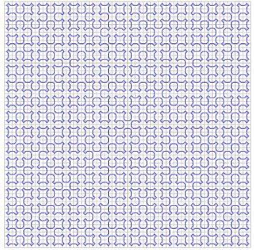
Fig. 12 Sierpinski curve
or, which is the same (for us), “ passing the triangle along Cesaro ”
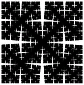
FIG. 13 Cesaro triangle, for clarity, the right angle is replaced by 85 ° - there should not be parameters in the numbering function, the curve should be uniform (accurate to symmetry). Because each such parameter makes the index not universal. Example: a combination of self-similar curves with a naive approach (taken here )
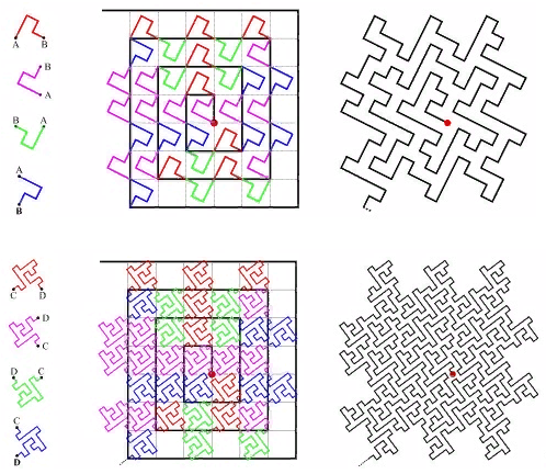
FIG. 14 “A Plane Filling Curve for the Year 2017”
And if the direction of rotation of the spiral can be attributed to symmetry, then the number of turns (at maximum extent) and the position of the center would have to be set by hand.
From the point of view of the perimeter of the pages, this, by the way, is a very good option, but the cost of computing such a function raises questions.
Isotropy is another important characteristic. It is understood that the numbering function should be easily generalizable to higher dimensions. And it’s good if for an N-dimensional cube all its N projections onto dimensions (N-1) are the same. This follows from the fact that we use isotropic space and it would be strange if different axes were used in functions differently.
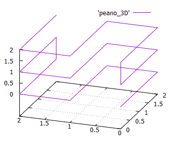
FIG. 15 Three-dimensional simplex 3x3x3 Peano curve
Isotropy is not a strict requirement, but it is an important indicator of the quality of a numbering curve.
Regarding continuity .
Above, we saw examples of continuous numbering functions that were not suitable for our purposes. On the other hand, the quite discontinuous line scan function with blocks is great for this (with some limitations). Not only that, if we built a block index based on continuous interlaced scanning, this would not change anything in terms of performance. Because if the block is read in whole, there is no difference in what order the objects will be received.
For self-similar curves this is also true.
- let's call the page size, the extent area of all objects on the disk page
- the characteristic size is the average page area
- on large requests (noticeably larger than the characteristic size), most of the objects are read using continuous reading of large blocks, and for continuous reading the order and discontinuity are not important. They are important only for peripheral pages that will be partially read. But the perimeter is generally the square root of the number of objects. And the cost of reading it can be neglected.
- on small queries - less than the characteristic size, the order of objects on the page does not matter since you still have to read it and this will be the main cost of the search.
- you should worry only about medium-sized queries, where the perimeter occupies a significant part of the search extent. For general reasons, a continuous numbering curve will arrange the data so that the search extent is located on fewer physical pages. Strictly speaking, no one has provided evidence of this, confirming the results of a numerical experiment are described here - the use of a (continuous) Hilbert curve gives 3 ... 10% less readings compared to the (discontinuous) Z-curve.
Percentage units are not something that will force us to abandon the study of discontinuous self-similar curves.
Simplexes
From what has been said, it follows that for the purposes of multidimensional indexing, only square (hypercubic) simplexes are recursively applied as many times as necessary (for sufficient detail of the lattice).
Yes, there are other self-similar ways to bridge a square lattice, however, there is no computationally cheap way to make such a transformation, including the reverse. Perhaps such numerical tricks exist, but they are not known to the author. In addition, square simplexes make it possible to effectively divide the search extent into subqueries by a cut along one of the coordinates . With a broken border between simplexes, this is impossible .
Why are simplexes square and not rectangular? For reasons of isotropy.
It remains to choose the appropriate size and numbering inside the simplex (bypass).
To choose the size of a simplex , you need to figure out what it affects. The number of generated subqueries that will have to be created during the search. For example, a simplex 3X3 of a Peano curve is cut into 3 subqueries with continuous intervals of numbers, first in X, and then each of them into 3 parts in Y. As a result, we return to the next stage of the recursion. If we had a similar (interlaced) simplex 5X5, it would have to be cut into 5 parts. Or into unequal parts (ex: 2 + 3), which is strange.
It reminds one of search trees in some ways - of course, you can use 5-decimal and 7-decimal trees, but in practice only binary ones are used. Trinity trees have their own narrow niche for searching by prefix. And this is not exactly what is intuitively understood as ternary trees.
This is explained by efficiency. In a ternary node, to select a descendant, one would have to make 2 comparisons. In a binary tree, this corresponds to a choice among 4 options. Even shorter tree depths do not block the loss of productivity from the increased number of comparisons.
In addition, if 3X3 were more effective than 2X2 simply because 3> 2, 4X4 would be more effective than 3X3, and 8X8 more effective than 5X5. You can always find a suitable power of two, which is formed by several iterations 2X2 ...
And what does bypassing a simplex affect? First of all, the number of subqueries generated by the search. Because it is good if the simplex allows you to cut yourself into pieces with continuous intervals of numbers. Here Peano 3X3 allows, so one iteration cuts it into 3 parts. And if you take an 8x8 simplex with a chess knight (Fig. 16), the only option is to immediately have 64 elements.

FIG. 16 One of the options for circumventing a simplex 8x8
So, since we found out that the optimal simplex is 2x2, we should consider what options exist for it.
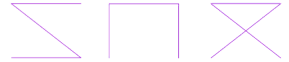
FIG. 17 Options for circumventing a 2x2 simplex
There are three of them, up to symmetry, conditionally called “Z”, “omega” and “alpha”.
It is immediately evident that the "alpha" crosses itself, and therefore is unsuitable for binary splitting. It would have to be cut immediately into 4 parts. Or 256 in the 8-dimensional case.
The ability to use a single algorithm for spaces of different dimensions (which we are deprived of in the case of a curve like “alpha”) looks very attractive. Therefore, in the future we will consider only the first two options.
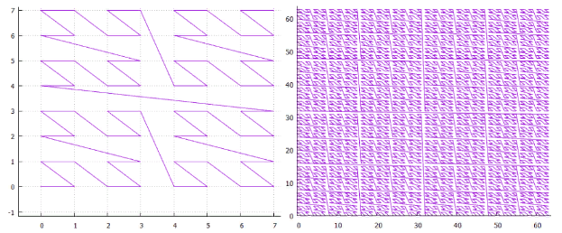
FIG. 18 Z-curve of
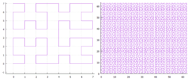
FIG. 19 “omega” - Hilbert curve.
Once these curves have a close kinship, theirmanages to process with one algorithm. The main specificity of the curve is localized in the splitting of the subquery.
- first we find the start extent, this is the minimum rectangle that includes the search extent and contains one continuous interval of key values.
It is found as follows -
- calculate the key values for the lower left and upper right points of the search extent (KMin, KMax)
- find the common binary prefix (from highs to lows) for KMin, KMax
- zeroing out all the digits after the prefix, we get SMin, filling them with units, we get SMax
- . , , SMin, . .
- , , ( ).
- Z- . z- — , — ( ). , , .
- calculate the key values for the lower left and upper right points of the search extent (KMin, KMax)
-
- , , . ,
- , . — “ ” >= “ ” () , “ ”
- “ ” > , ,
- , ,
- “ ” > , , ,
- “ ” == ,
- “ ” > , ,
-
- 0 1 —
- 0 1 —
- , , 1, 0. .
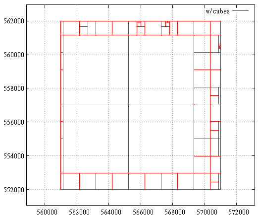
FIG. 20 is a subquery for the Z-curve of
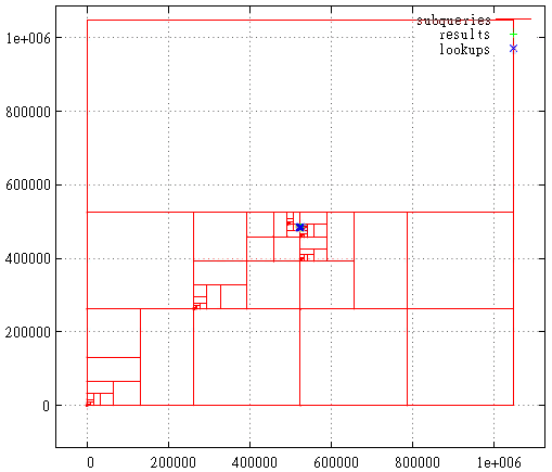
FIG. 21 Hilbert curve, the case when the starting extent is maximum
. The first stage is shown here - cutting off the excess layer from the maximum extent.

FIG. 22 Hilbert curve, search query area
And here is a breakdown into subqueries, points found and index calls in the search query area. This is still a very unsuccessful request from the point of view of the Hilbert curve. Usually everything is much less bloody.
However, query statistics say that (roughly) on the same data, a two-dimensional index based on a Hilbert curve reads 5% less disk pages on average, but it works half slower. The slowdown is also caused by the fact that the calculation itself (direct and inverse) of this curve is much harder - 2000 processor cycles for Hilbert compared to 50 for the Z-curve.
Having ceased to support the Hilbert curve, it would be possible to simplify the algorithm; at first glance, such a slowdown is not justified. On the other hand, this is just a two-dimensional case, for example, in 8-dimensional space or more, statistics can sparkle with completely new colors. This issue is still awaiting clarification.
PS: The Z-curve is sometimes called the bit-interleaving curve due to the algorithm for calculating the value - the digits of each coordinate fall into the key value through one, which is very technological. But you can after all interleave the discharges not individually, but in packs of 2.3 ... 8 ... pieces. Now, if we take 8 bits, then on a 32-bit key we get an analogue of the 4-level GRID index from MS SQL. And in an extreme case - one pack of 32 bits each - the horizontal scanning algorithm.
Such an index (not lowercase, of course) can be very effective, even more efficient than the Z-curve on some data sets. Unfortunately, due to loss of generality.
PPS : The described index is very similar to working with a quad tree. The maximum extent is the root page of the quad tree, it has 4 descendants ... And therefore, the algorithm can be attributed to “direct access methods”.
The differences are still fundamental.
The quad tree is not stored anywhere, it is virtual, embedded in the very nature of numbers. There are no restrictions on the depth of the tree; we obtain information on the population of descendants from the population of the main tree. Moreover, the main tree is read once, we go from the smallest to the oldest values. It's funny, but the physical structure of the B-tree makes it possible to avoid empty queries and limit the recursion depth.
One more thing - at each iteration only two descendants appear - from them 4 subqueries can be generated, and can be not generated if there is no data under them. In the 3-dimensional case we would talk about 8 descendants, in the 8-dimensional case - about 256.
PPPS: at the beginning of this article, we talked about dichotomy when searching in a multidimensional index - in order to get the logarithmic value, it is necessary to divide some finite resource at either iteration — either the key value space or the search space. In the presented algorithm, this dichotomy collapsed - we simultaneously share both the key and the space.
“I live in both yards, and my trees are always taller.” ( C )
PPPPS : Once you call the Z-curve, here you have the Z-order and bit-interleaving and the Morton code / curve. And also it is known as the Lebesgue curve, so in order to maintain balance, the author entitled the article, including in honor of Henry Leon Lebesgue .
PPPPPS : In the title illustration, a view ofFedchenko Glacier , just beautiful, and there is enough emptiness. In fact, the author was impressed with how different ideas and methods smoothly flow into each other, gradually merging into one algorithm. Just as the many small water sources that make up the catchment basin form a single runoff.
All Articles