Discrete mathematics for WMS: algorithm for compressing goods in cells (part 2)
In the article, we will describe how we developed an algorithm for the optimal compression of the remaining goods in cells. We’ll tell you how to choose the necessary metaheuristics of the framework zoo environment: taboo search, genetic algorithm, ant colony, etc.
We will conduct a computational experiment to analyze the operating time and accuracy of the algorithm. We summarize and summarize the valuable experience gained in solving this problem of optimization and implementation of “smart technologies” in the customer’s business processes.
The article will be useful to those who implement intelligent technologies, work in the warehouse or production logistics industry, as well as programmers who are interested in mathematics applications in business and process optimization in the enterprise.
Introductory part
This publication continues the series of articles in which we share our successful experience in implementing optimization algorithms in warehouse processes. Previous publications:
- clustering algorithm for consignments in stock.
- an algorithm for compressing residual goods in cells (part 1).
How to read an article. If you read the previous articles, you can immediately proceed to the chapter "Development of an algorithm for solving the problem", if not, then the description of the problem to be solved in the spoiler is below.
Description of the problem to be solved at the customer’s warehouse
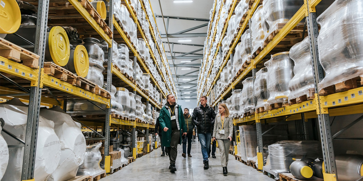
In 2018, we made a project to introduce a WMS system at the warehouse of the LD Trading House company in Chelyabinsk. Introduced the product “1C-Logistics: Warehouse Management 3” for 20 jobs: WMS operators, storekeepers, forklift drivers. Warehouse average of about 4 thousand m2, the number of cells 5000 and the number of SKU 4500. The warehouse stores ball valves of their own production in different sizes from 1 kg to 400 kg. Inventories are stored in the context of batches due to the need to select goods according to FIFO and the "in-line" specifics of product placement (explanation below).
When designing automation schemes for warehouse processes, we were faced with the existing problem of non-optimal storage of stocks. Stacking and storage of cranes has, as we have already said, “in-line” specifics. That is, the products in the cell are stacked in rows one on top of the other, and the ability to put a piece on a piece is often absent (they simply fall, and the weight is not small). Because of this, it turns out that only one nomenclature of one batch can be in one piece storage unit;
Products arrive at the warehouse daily and each arrival is a separate batch. In total, as a result of 1 month of warehouse operation, 30 separate lots are created, despite the fact that each should be stored in a separate cell. The goods are often taken not in whole pallets, but in pieces, and as a result, in the piece selection area, in many cells the following picture is observed: in a cell with a volume of more than 1 m3 there are several pieces of cranes that occupy less than 5-10% of the cell volume (see Fig. 1 )
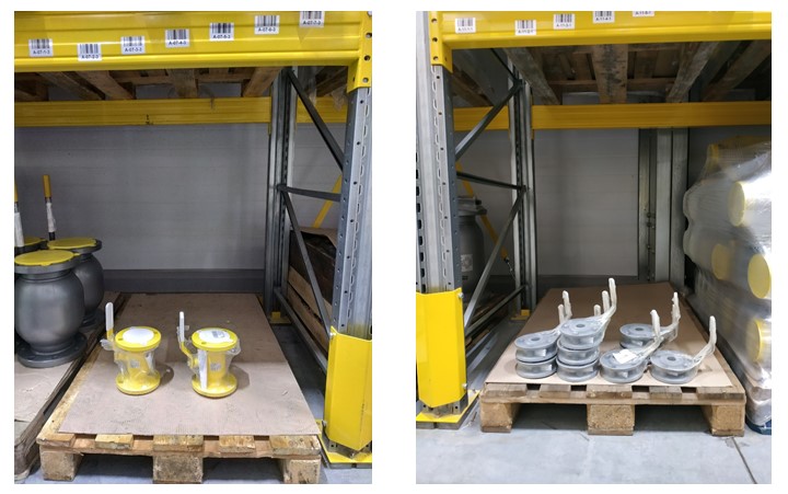
Fig 1. Photo of several pieces in a cell
On the face of the suboptimal use of storage capacity. To imagine the scale of the disaster, I can cite the figures: on average there are between 100 and 300 cells of such cells with a "scanty" residue in different periods of the warehouse’s operation. Since the warehouse is relatively small, in the warehouse loading seasons this factor becomes a “bottleneck” and greatly inhibits the warehouse processes of acceptance and shipment.
The idea came up: to bring the balances with the closest dates to one single lot and place such balances with a unified batch compactly together in one cell, or in several if there isn’t enough space in one to accommodate the total number of balances. An example of such a “compression” is shown in Figure 2.
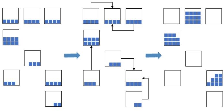
Fig. 2. Cell compression scheme
This allows you to significantly reduce the occupied warehouse space, which will be used for the newly placed goods. In the situation of overloading warehouse capacities, such a measure is extremely necessary, otherwise there may simply not be enough free space for placing new goods, which will lead to a stopper in the warehouse processes of placement and replenishment and, as a result, a stopper for acceptance and shipment. Previously, before the WMS system was implemented, such an operation was performed manually, which was not effective, since the process of finding suitable residues in the cells was quite long. Now, with the introduction of WMS systems, they decided to automate the process, speed it up and make it intelligent.
The process of solving this problem is divided into 2 stages:
In the current article, we finish with a description of the second stage of the solution process and consider directly the optimization algorithm itself.
Process bottleneck
In 2018, we made a project to introduce a WMS system at the warehouse of the LD Trading House company in Chelyabinsk. Introduced the product “1C-Logistics: Warehouse Management 3” for 20 jobs: WMS operators, storekeepers, forklift drivers. Warehouse average of about 4 thousand m2, the number of cells 5000 and the number of SKU 4500. The warehouse stores ball valves of their own production in different sizes from 1 kg to 400 kg. Inventories are stored in the context of batches due to the need to select goods according to FIFO and the "in-line" specifics of product placement (explanation below).
When designing automation schemes for warehouse processes, we were faced with the existing problem of non-optimal storage of stocks. Stacking and storage of cranes has, as we have already said, “in-line” specifics. That is, the products in the cell are stacked in rows one on top of the other, and the ability to put a piece on a piece is often absent (they simply fall, and the weight is not small). Because of this, it turns out that only one nomenclature of one batch can be in one piece storage unit;
Products arrive at the warehouse daily and each arrival is a separate batch. In total, as a result of 1 month of warehouse operation, 30 separate lots are created, despite the fact that each should be stored in a separate cell. The goods are often taken not in whole pallets, but in pieces, and as a result, in the piece selection area, in many cells the following picture is observed: in a cell with a volume of more than 1 m3 there are several pieces of cranes that occupy less than 5-10% of the cell volume (see Fig. 1 )
Fig 1. Photo of several pieces in a cell
On the face of the suboptimal use of storage capacity. To imagine the scale of the disaster, I can cite the figures: on average there are between 100 and 300 cells of such cells with a "scanty" residue in different periods of the warehouse’s operation. Since the warehouse is relatively small, in the warehouse loading seasons this factor becomes a “bottleneck” and greatly inhibits the warehouse processes of acceptance and shipment.
Idea of solving a problem
The idea came up: to bring the balances with the closest dates to one single lot and place such balances with a unified batch compactly together in one cell, or in several if there isn’t enough space in one to accommodate the total number of balances. An example of such a “compression” is shown in Figure 2.
Fig. 2. Cell compression scheme
This allows you to significantly reduce the occupied warehouse space, which will be used for the newly placed goods. In the situation of overloading warehouse capacities, such a measure is extremely necessary, otherwise there may simply not be enough free space for placing new goods, which will lead to a stopper in the warehouse processes of placement and replenishment and, as a result, a stopper for acceptance and shipment. Previously, before the WMS system was implemented, such an operation was performed manually, which was not effective, since the process of finding suitable residues in the cells was quite long. Now, with the introduction of WMS systems, they decided to automate the process, speed it up and make it intelligent.
The process of solving this problem is divided into 2 stages:
- at the first stage, we find groups of parties that are close in date for compression (this is the first article for this dedication task);
- at the second stage, for each group of batches we calculate the most compact placement of product residues in cells.
In the current article, we finish with a description of the second stage of the solution process and consider directly the optimization algorithm itself.
Development of an algorithm for solving the problem
Before proceeding with a direct description of the optimization algorithm, it is necessary to talk about the main criteria for the development of such an algorithm, which were set as part of the WMS- system implementation project.
- First, the algorithm should be easy to understand . This is a natural requirement, since it is assumed that the algorithm will be supported and further developed by the customer’s IT service in the future, which is often far from mathematical subtleties and wisdom.
- Secondly, the algorithm should be fast . Almost all goods in the warehouse are involved in the compression procedure (this is about 3,000 items) and for each product it is necessary to solve a dimension problem of approximately 10x100.
- Thirdly, the algorithm must calculate solutions close to optimal .
- Fourth, the time for designing, implementing, debugging, analyzing and internal testing the algorithm is relatively small. This is an essential requirement, since the project budget , including for this task, was limited .
It is worth saying that to date, mathematicians have developed many effective algorithms to solve the Single-Source Capacitated Facility Location Problem problem. Consider the main varieties of the available algorithms.
Some of the most efficient algorithms are based on the approach of the so-called Lagrange relaxation. As a rule, these are rather complex algorithms that are difficult to understand for a person who is not immersed in the intricacies of discrete optimization. The "black box" with complex, but effective algorithms of Lagrange relaxation of the customer did not suit.
There are quite effective metaheuristics (what is metaheuristics read here , what is heuristics read here ), for example, genetic algorithms, annealing simulation algorithms, ant colony algorithms, Tabu search algorithms and others (an overview of such metaheuristics in Russian can be found here ). But such algorithms have already satisfied the customer, since:
- Able to calculate solutions to problems that are very close to optimal.
- Simple enough to understand, further support, debug and refine.
- They can quickly calculate a solution to a problem.
It was decided to use metaheuristics. Now it remained to choose one “framework” among the large “zoo” of famous metaheuristics for solving the Single-Source Capacitated Facility Location Problem. After reading a series of articles that analyzed the effectiveness of various metaheuristics, our choice fell on the GRASP algorithm, as compared with other metaheuristics, it showed rather good results on the accuracy of the calculated solutions to the problem, was one of the fastest and, most importantly, it had the simplest and transparent logic.
The scheme of the GRASP algorithm in relation to the Single-Source Capacitated Facility Location Problem task is described in detail in the article . The general scheme of the algorithm is as follows.
- Stage 1. Generate some feasible solution to the problem by a greedy randomized algorithm.
- Stage 2. Improve the resulting solution in stage 1 using the local search algorithm in a number of neighborhoods.
- If the stop condition is fulfilled, then complete the algorithm, otherwise go to step 1. The solution with the lowest total cost among all the solutions found will be the result of the algorithm.
The condition for stopping the algorithm can be a simple restriction on the number of iterations or a restriction on the number of iterations without any improvement in the solution.
The code of the general scheme of the algorithm
int computeProblemSolution(int **aCellsData, int **aMatDist, int cellsNumb, int **aMatSolution, int **aMatAssignmentSolution) { // // int . WMS 3 ( ., 10 ), // aMatSolutionIteration - : // [i][0] , [i][1] , [i][2] // [i][3] int **aMatSolutionIteration = new int*[cellsNumb]; for (int count = 0; count < cellsNumb; count++) aMatSolutionIteration[count] = new int[4]; // aMatAssignmentSolutionIteration - . [i][j] = 1 - j i, 0 int **aMatAssignmentSolutionIteration = new int*[cellsNumb]; for (int count = 0; count < cellsNumb; count++) aMatAssignmentSolutionIteration[count] = new int[cellsNumb]; const int maxIteration = 10; int iter = 0, recordCosts = 1000000; // , int totalDemand = 0; for (int i = 0; i < cellsNumb; i++) totalDemand += aCellsData[i][1]; while (iter < maxIteration) { // setValueIn2Array(aMatAssignmentSolutionIteration, cellsNumb, cellsNumb, 0); // setClearSolutionArray(aMatSolutionIteration, cellsNumb, 4); // int *aFreeContainersFitnessFunction = new int[cellsNumb]; // , findGreedyRandomSolution(aCellsData, aMatDist, cellsNumb, aMatSolutionIteration, aMatAssignmentSolutionIteration, aFreeContainersFitnessFunction, false); // improveSolutionLocalSearch(aCellsData, aMatDist, cellsNumb, aMatSolutionIteration, aMatAssignmentSolutionIteration, totalDemand); // ( ) bool feasible = isSolutionFeasible(aMatSolutionIteration, aCellsData, cellsNumb); // , if (feasible == false) { getFeasibleSolution(aCellsData, aMatDist, cellsNumb, aMatSolutionIteration, aMatAssignmentSolutionIteration); } // , , int totalCostsIteration = getSolutionTotalCosts(aMatSolutionIteration, cellsNumb); if (totalCostsIteration < recordCosts) { recordCosts = totalCostsIteration; copy2Array(aMatSolution, aMatSolutionIteration, cellsNumb, 3); } iter++; } delete2Array(aMatSolutionIteration, cellsNumb); delete2Array(aMatAssignmentSolutionIteration, cellsNumb); return recordCosts; }
Let us consider in more detail the operation of the greedy randomized algorithm at stage 1. It is believed that at the beginning not a single cell-container is selected.
- Step 1. For each container cell not currently selected, the value is calculated cost formula
Where - the amount of the cost of choosing a container and the total cost of moving goods from cells that are not yet attached to any container into the container . Such cells are selected so that the total volume of goods in them does not exceed the capacity of the container . Donor cells are sequentially selected to move into a container container in order of increasing cost of moving the quantity of goods into the container . Cell selection is carried out until the container capacity is exceeded. - Step 2. A lot is formed containers with function value not exceeding the threshold value where in our case it is 0.2.
- Step 3. Randomly from the set container is selected . cells that were previously selected in the container in step 1, they are finally assigned to such a container and do not further participate in the calculations of the greedy algorithm.
- Step 4. If all donor cells are assigned to containers, the greedy algorithm stops its work, otherwise it goes back to step 1.
The randomized algorithm at each iteration tries to construct the solution in such a way that there is a balance between the quality of the solutions it constructs, as well as their diversity. These two requirements for starting decisions are the key conditions for the successful operation of the algorithm, since:
- if the solutions are of poor quality, then the subsequent improvement in stage 2 will not give significant results, since even improving the bad solutions, we will very often get the same poor quality solutions;
- If all the solutions are good, but the same, then the local search procedures will converge to the same solution, it is by no means a fact that the optimal one. This effect is called hitting a local minimum and should always be avoided.
Greedy randomized algorithm code
void findGreedyRandomSolution(int **aCellsData, int **aMatDist, int cellsNumb, int **aMatSolutionIteration, int **aMatAssignmentSolutionIteration, int *aFreeContainersFitnessFunction, bool isOldSolution) { // int numCellsInSolution = 0; if (isOldSolution) { // , aFreeContainersFitnessFunction // numCellsInSolution , for (int i = 0; i < cellsNumb; i++) { for (int j = 0; j < cellsNumb; j++) { if (aMatAssignmentSolutionIteration[i][j] == 1) numCellsInSolution++; } } } // , aFreeContainersFitnessFunction, // [i][j] = 1, j i, 0 int **aFreeContainersAssigntCells = new int*[cellsNumb]; for (int count = 0; count < cellsNumb; count++) aFreeContainersAssigntCells[count] = new int[cellsNumb]; while (numCellsInSolution != cellsNumb) { setValueIn2Array(aFreeContainersAssigntCells, cellsNumb, cellsNumb, 0); // // setFreeContainersFitnessFunction(aCellsData, aMatDist, cellsNumb, aFreeContainersFitnessFunction, aFreeContainersAssigntCells); // , // , int selectedRandomContainer = selectGoodRandomContainer(aFreeContainersFitnessFunction, cellsNumb); // aMatSolutionIteration[selectedRandomContainer][0] = selectedRandomContainer; aMatSolutionIteration[selectedRandomContainer][1] = 0; aMatSolutionIteration[selectedRandomContainer][2] = aCellsData[selectedRandomContainer][2]; for (int j = 0; j < cellsNumb; j++) { if (aFreeContainersAssigntCells[selectedRandomContainer][j] == 1) { aMatAssignmentSolutionIteration[selectedRandomContainer][j] = 1; aMatSolutionIteration[selectedRandomContainer][1] += aCellsData[j][1]; aMatSolutionIteration[selectedRandomContainer][2] += aMatDist[selectedRandomContainer][j]; aMatSolutionIteration[selectedRandomContainer][3] = 0; aFreeContainersFitnessFunction[j] = 10000; numCellsInSolution++; } } } delete2Array(aFreeContainersAssigntCells, cellsNumb); delete[] aFreeContainersFitnessFunction; } void setFreeContainersFitnessFunction(int **aCellsData, int **aMatDist, int cellsNumb, int *aFreeContainersFitnessFunction, int **aFreeContainersAssigntCells) { // , i // [0][k] - , [1][k] - int **aCurrentDist = new int*[2]; for (int count = 0; count < 2; count++) aCurrentDist[count] = new int[cellsNumb]; for (int i = 0; i < cellsNumb; i++) { // 10000 - , if (aFreeContainersFitnessFunction[i] >= 10000) continue; // int containerCurrentVolume = aCellsData[i][1]; // int containerCosts = aCellsData[i][2]; // -, i int amountAssignedCell = 0; setCurrentDist(aMatDist, cellsNumb, aCurrentDist, i); for (int j = 0; j < cellsNumb; j++) { int currentCell = aCurrentDist[1][j]; if (currentCell == i) continue; if (aFreeContainersFitnessFunction[currentCell] >= 10000) continue; if (aCellsData[i][0] < containerCurrentVolume + aCellsData[currentCell][1]) continue; aFreeContainersAssigntCells[i][currentCell] = 1; containerCosts += aCurrentDist[0][j]; containerCurrentVolume += aCellsData[currentCell][1]; amountAssignedCell++; } // ( ) if (aCellsData[i][1] > 0) { aFreeContainersAssigntCells[i][i] = 1; amountAssignedCell++; } // 1 ( ), // 1. // . , // ( ) . // ( ), // , . if (amountAssignedCell > 1) amountAssignedCell *= 10; if (amountAssignedCell > 0) aFreeContainersFitnessFunction[i] = containerCosts / amountAssignedCell; else aFreeContainersFitnessFunction[i] = 10000; } delete2Array(aCurrentDist, 2); } int selectGoodRandomContainer(int *aFreeContainersFitnessFunction, int cellsNumb) { int minFit = 10000; for (int i = 0; i < cellsNumb; i++) { if (minFit > aFreeContainersFitnessFunction[i]) minFit = aFreeContainersFitnessFunction[i]; } int threshold = minFit * (1.2); // 20 % // int *aFreeContainersThresholdFitnessFunction = new int[cellsNumb]; int containerNumber = 0; for (int i = 0; i < cellsNumb; i++) { if (threshold >= aFreeContainersFitnessFunction[i] && aFreeContainersFitnessFunction[i] < 10000) { aFreeContainersThresholdFitnessFunction[containerNumber] = i; containerNumber++; } } int randomNumber = rand() % containerNumber; int randomContainer = aFreeContainersThresholdFitnessFunction[randomNumber]; delete[] aFreeContainersThresholdFitnessFunction; return randomContainer; }
After the “starting” solution is constructed in stage 1, the algorithm proceeds to stage 2, where the improvement of such a found solution is carried out, where improvement naturally means reducing the total cost. The logic of the local search algorithm in step 2 is as follows.
- Step 1. For the current solution all "neighboring" solutions are constructed according to some kind of neighborhood , , ..., and for each "neighboring" solution, the value of the total costs is calculated.
- Step 2. If among the neighboring solutions there was a better solution than the original solution then assumed equal and the algorithm proceeds to step 1. Otherwise, if among the neighboring solutions there was no better solution than the original one, then the view of the neighborhood changes to a new one that has not been previously considered, and the algorithm proceeds to step 1. If all available views of the neighborhood are considered, but failed find a better solution than the original, the algorithm ends its work.
Views of the surroundings are selected sequentially from the following stack: , , , , . Views of the surrounding area are divided into 2 types: the first type (neighborhood , , ), where many containers do not change, but only the options for attaching donor cells change; second type (neighborhood , ), where not only the options for attaching cells to containers change, but also the many containers themselves.
We denote - the number of elements in the set . The figures below depict options for neighborhoods of the first type .

Fig. 7. Neighborhood
Neighborhood (or shift neighborhood): contains all the options for solving the problem that differ from the original by changing the attachment of only one donor cell to the container. The size of the neighborhood is not more options.
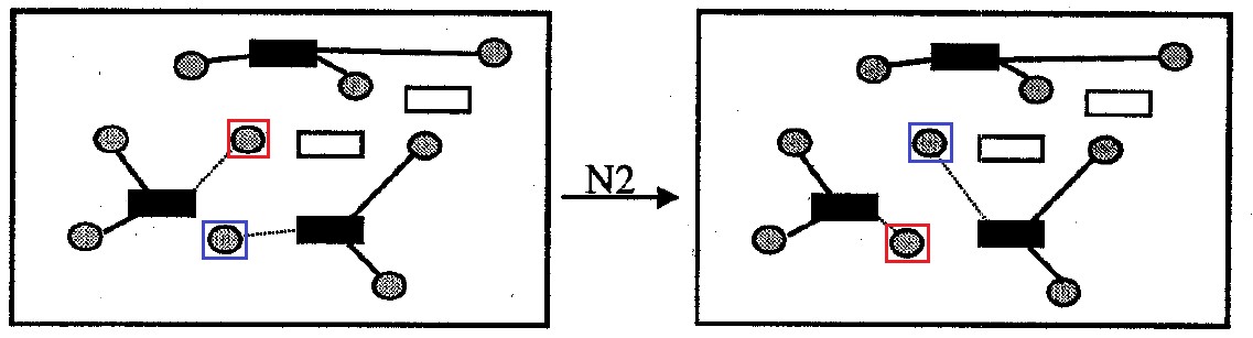
Fig. 8. Neighborhood
The code of the local search algorithm in the neighborhood of N1
void findBestSolutionInNeighborhoodN1(int **aCellsData, int **aMatDist, int cellsNumb, int **aMatSolutionIteration, int **aMatAssignmentSolutionIteration, int totalDemand, bool stayFeasible) { // int recordDeltaCosts, recordCell, recordNewContainer, recordNewCosts, recordNewPenalty, recordOldContainer, recordOldCosts, recordOldPenalty; do { recordDeltaCosts = 10000; int totalContainersCapacity = 0; for (int i = 0; i < cellsNumb; i++) if (aMatSolutionIteration[i][1] > 0) totalContainersCapacity += aCellsData[i][0]; // - for (int j = 0; j < cellsNumb; j++) { // , j int currentContainer; for (int i = 0; i < cellsNumb; i++) { if (aMatAssignmentSolutionIteration[i][j] == 1) { currentContainer = i; break; } } // , j ( ) int numbAssignedCells = 0; if (aMatSolutionIteration[j][0] >= 0) { for (int i = 0; i < cellsNumb; i++) { if (aMatAssignmentSolutionIteration[j][i] == 1) { numbAssignedCells = i; } } } else { numbAssignedCells = 0; } // j , j, // "" , if (j == currentContainer && numbAssignedCells > 1) { continue; } // int currentTotalContainersCapacity = totalContainersCapacity - aCellsData[currentContainer][0]; // , , j int currentCosts = aMatDist[currentContainer][j]; // j , if (aMatSolutionIteration[currentContainer][1] - aCellsData[j][1] == 0) currentCosts += aCellsData[currentContainer][2]; // j , int currentPenelty = getPenaltyValueForSingleCell(aCellsData, aMatSolutionIteration, currentContainer, j, 0); currentCosts += currentPenelty; for (int i = 0; i < cellsNumb; i++) { if (i == currentContainer) continue; if (stayFeasible) { if (max(0, aMatSolutionIteration[i][1]) + aCellsData[j][1] > aCellsData[i][0]) continue; } else { if (currentTotalContainersCapacity + aCellsData[i][0] < totalDemand) continue; } // int newCosts = aMatDist[i][j]; // if (aMatSolutionIteration[i][0] == -1) newCosts += aCellsData[i][2]; // int newPenalty = getPenaltyValueForSingleCell(aCellsData, aMatSolutionIteration, i, j, 1); newCosts += newPenalty; int deltaCosts = newCosts - currentCosts; if (deltaCosts < 0 && deltaCosts < recordDeltaCosts) { recordDeltaCosts = deltaCosts; recordCell = j; recordNewContainer = i; recordNewCosts = newCosts; recordNewPenalty = newPenalty; recordOldContainer = currentContainer; recordOldCosts = currentCosts; recordOldPenalty = currentPenelty; } } } // , if (recordDeltaCosts < 0) { // aMatSolutionIteration[recordOldContainer][1] -= aCellsData[recordCell][1]; aMatSolutionIteration[recordOldContainer][2] -= recordOldCosts; if (aMatSolutionIteration[recordOldContainer][1] == 0) aMatSolutionIteration[recordOldContainer][0] = -1; aMatSolutionIteration[recordOldContainer][3] -= recordOldPenalty; aMatAssignmentSolutionIteration[recordOldContainer][recordCell] = 0; // aMatSolutionIteration[recordNewContainer][1] += aCellsData[recordCell][1]; aMatSolutionIteration[recordNewContainer][2] += recordNewCosts; if (aMatSolutionIteration[recordNewContainer][0] == -1) aMatSolutionIteration[recordNewContainer][0] = recordNewContainer; aMatSolutionIteration[recordNewContainer][3] += recordNewPenalty; aMatAssignmentSolutionIteration[recordNewContainer][recordCell] = 1; //checkCorrectnessSolution(aCellsData, aMatDist, aMatAssignmentSolutionIteration, aMatSolutionIteration, cellsNumb); } } while (recordDeltaCosts < 0); }
Neighborhood (or swap neighborhood): contains all the options for solving the problem that differ from the original one by the mutual exchange of attachment to containers for one pair of donor cells. Neighborhood size no more options.
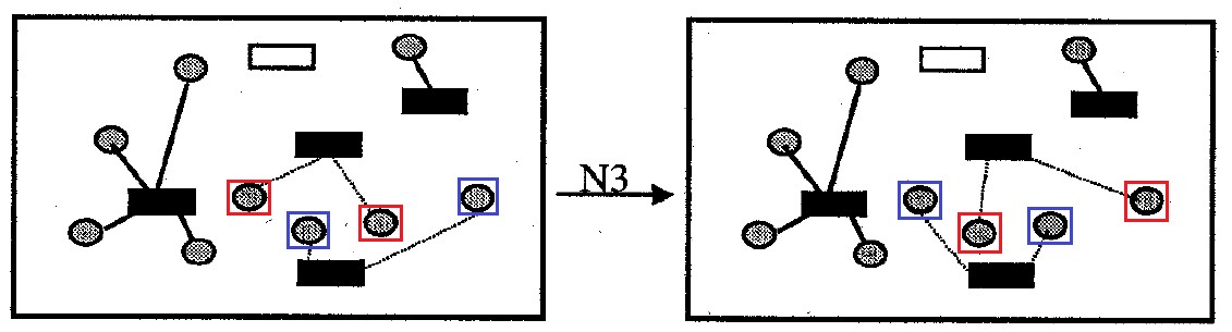
Fig. 9. Neighborhood
Neighborhood : contains all the options for solving the problem, which differ from the original one by mutual replacement of the attachment of all cells for one pair of containers. Neighborhood size no more options.
The second type of neighborhoods is considered as a mechanism of "diversification" of decisions, when it is no longer possible to obtain improvements by searching the "close" neighborhoods of the first type.
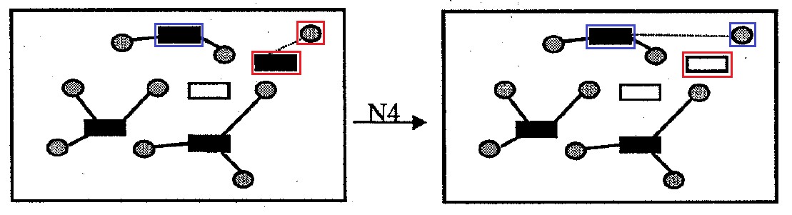
Fig. 10. Neighborhood
Neighborhood : contains all the options for solving the problem that differ from the original one by removing one container cell from the solution. Donor cells that were attached to such a container that was removed from the solution are attached to other containers in order to minimize the amount of transportation costs and the penalty for exceeding the capacity of the container. Neighborhood size no more options.

Fig. 11. Neighborhood
Neighborhood : contains all the options for solving the problem that differ from the original one by detaching cells from one container and attaching such cells to another empty container for an arbitrary one pair of containers. The size of the neighborhood is not more options.
The authors of the article say that, based on the results of computational experiments, the best option is to first search for “near” neighborhoods of the first type, and then search for “distant” neighborhoods.
Note that the authors of the article recommend doing a search in the vicinity without taking into account restrictions on the capacity of each container. Instead, if the capacity of the container is exceeded, then add to the total cost of the solution some positive amount of “fine”, which will impair the attractiveness of such a solution compared to other solutions. The only restriction is placed on the total volume of containers, that is, the total volume of goods transported from donor cells should not exceed the total capacity of the containers. This removal of restrictions is done because if restrictions are taken into account, then often the neighborhood will not contain a single acceptable solution and the local search algorithm will finish its work immediately after its start, without making any improvements. Figure 12 shows an example of a local search operation without taking into account restrictions on the capacity of each container.

Fig. 12. The work of local search without taking into account restrictions on the capacity of each container
In this figure, it is assumed that the red and green residues from some donor cells are not beneficial to move to any other container except the second. This means that further improvement of the solution is impossible, since any other new feasible solution to the problem, where the restrictions on capacity are respected, will be worse than the original in terms of transportation costs. As you can see, the algorithm for 2 iterations builds a feasible solution much better than the original, despite the fact that the first iteration builds an invalid solution with excess capacity.
Note that this approach of introducing a “penalty” for the inadmissibility of a solution is quite common in discrete optimization and is often used in algorithms such as genetic algorithms, taboo search, etc.
After the local search algorithm is completed, if the solution found is still unacceptable, that is, the container capacity limits have been exceeded somewhere, we must bring the solution found to an acceptable form, where all restrictions on container capacity are respected. The algorithm for eliminating the inadmissibility of the solution is as follows.
- Step 1. Perform a local search on the neighborhoods of shift and swap . In this case, the transition is carried out only in those decisions that reduce exactly the amount of “fine”. If it is not possible to reduce the fine, then a solution with lower total costs is chosen. If further improvement by local search is not at all possible, go to step 2, otherwise, if the resulting solution is valid, then complete the algorithm.
- Step 2. If the solution is still unacceptable, then from each container where there was an excess of capacity, donor cells are detached in order of increasing volume of goods until the restriction on capacity is met. For such detached cells, all steps of the algorithm, starting from the first, are repeated, despite the fact that the many available selected containers and the method of attaching the remaining cells to them are fixed and cannot be changed. Note that such a step 2, as the computational experiment shows, is required to be performed extremely rarely.
Computational experiment and analysis of algorithm efficiency
The GRASP algorithm was implemented from scratch in C ++ , since we did not find the source code for the algorithm described in the article . The program code was compiled using g ++ with the -O2 optimization option.
Visual Studio project code has been uploaded to GitHub . The only thing the customer asked was to remove some of the most complex local search procedures for reasons of intellectual property, trade secrets, etc.
In the article that describes the GRASP algorithm, its high efficiency was stated, where by efficiency it is meant that it stably calculates solutions very close to optimal, and that it works quite quickly. In order to verify the real effectiveness of such a GRASP algorithm, we conducted our own computational experiment. The input data of the problem was generated by us randomly with a uniform distribution. The solutions calculated by the algorithm were compared with the optimal solutions, which were calculated by the exact algorithm proposed in the article . Sources of such an exact algorithm are available on GitHub by reference . The dimension of the task, for example, 10x100 will mean that we have 10 donor cells and 100 container cells.
The calculations were carried out on a personal computer with the following characteristics: CPU 2.50 GHz, Intel Core i5-3210M, 8 GB RAM, operating system Windows 10 (x64).
| Task dimension | amount
generated | Average time
GRASP | Average time
|
GRASP, % |
|---|---|---|---|---|
| 550 | 50 | 0.08 | 1,22 | 0.2 |
| 1050 | 50 | 0.14 | 3,75 | 0,4 |
| 10100 | 50 | 0.55 | 15,81 | 1.4 |
| 10200 | 25 | 2.21 | 82.73 | 1.8 |
| 20x100 | 25 | 1.06 | 264.15 | 2,3 |
| 20x200 | 25 | 4.21 | 797.39 | 2.7 |
As can be seen from table 3, the GRASP algorithm really calculates close to optimal solutions, and with an increase in the dimension of the problem, the quality of the algorithm solutions deteriorates slightly. It is also seen from the experimental results that the GRASP algorithm is quite fast, for example, it solves a 10x100 dimension problem on average in 0.5 seconds. It should be noted at last that the results of our computational experiment are consistent with the results in the article .
Running the algorithm in production
After the algorithm was developed, debugged and tested in a computational experiment, the time came to put it into operation. The algorithm was implemented in C ++ and was placed in a DLL that connected to the 1C application as an external component of the Native type. Read about what external 1C components are and how to properly develop and connect them to the 1C application here . In the program “1C: Warehouse Management 3”, a processing form was developed in which the user can start the procedure for compressing residuals with the parameters he needs. A screenshot of the form is shown below.

Fig. 13. The form of the procedure for “compression” of balances in Appendix 1C: Warehouse Management 3
The user can select the compression parameters for residues in the form:
- Compression mode: with batch clustering (see the first article) and without it.
- Warehouse, in the cells of which it is necessary to carry out compression. In one room there can be several warehouses for different organizations. Just such a situation was with our client.
- Also, the user can interactively adjust the quantity of goods transferred from the donor cell to the container and delete the item from the list for compression, if for some reason he wants it to not participate in the compression procedure.
Conclusion
At the end of the article, I would like to summarize the experience gained as a result of the introduction of such an optimization algorithm.
- . : , , . - :
- , ;
- .
- ( ), , . «», - . , , . , , , - , .
- , ( ), . , , . , . . , .
- :
- .
- .
- . , .
- . , . , , , , .
- , . ( ) . , .
- .
And, I think, the most important thing. The optimization process in the enterprise often must follow after the completion of the informatization process. Optimization without preliminary informatization is of little use , since there is nowhere to get data from and there is nowhere to write the data of the algorithm solution. I think that most medium-sized and large domestic enterprises have closed the basic needs for automation and informatization and are ready for more “fine-tuning” of process optimization.
Therefore, we practice after the implementation of the information system, be it ERP, WMS, TMS, etc. make small extra. projects to optimize those processes that were identified during the implementation of the information system as problematic and important for the client. I think this is a promising practice that will gain momentum in the coming years.
, ,
, .
All Articles