Discrete mathematics for WMS: algorithm for compressing goods in cells (part 1)
In the article, we will tell you how to solve the problem of the lack of free cells in the warehouse and the development of a discrete optimization algorithm to solve this problem. We will talk about how we “built” the mathematical model of the optimization problem, and about what difficulties we suddenly encountered when processing the input data for the algorithm.
If you are interested in mathematical applications in business and you are not afraid of hard identical transformations of formulas at the 5th grade level, then welcome to cat!
The article will be useful to those who implement WMS systems, work in the warehouse or production logistics industry, as well as programmers who are interested in mathematics applications in business and process optimization in the enterprise.
Introductory part
This publication continues the series of articles in which we share our successful experience in implementing optimization algorithms in warehouse processes.
The previous article described the specifics of the warehouse in which we introduced the WMS system, and also explained why we needed to solve the problem of clustering batches of goods leftovers during the implementation of the WMS system, and how we did it.
When we finished writing an article on optimization algorithms, it turned out to be very large, so we decided to divide the accumulated material into 2 parts:
- In the first part (this article) we will talk about how we “built” the mathematical model of the problem, and about what great difficulties we suddenly encountered when processing and converting input data for the algorithm.
- In the second part, we will examine in detail the implementation of the algorithm in C ++ , conduct a computational experiment and summarize the experience that we gained during the implementation of such “intelligent technologies” in the customer’s business processes.
How to read an article. If you read the previous article, you can immediately go to the chapter "Overview of existing solutions", if not, then the description of the problem to be solved in the spoiler below.
Process bottleneck
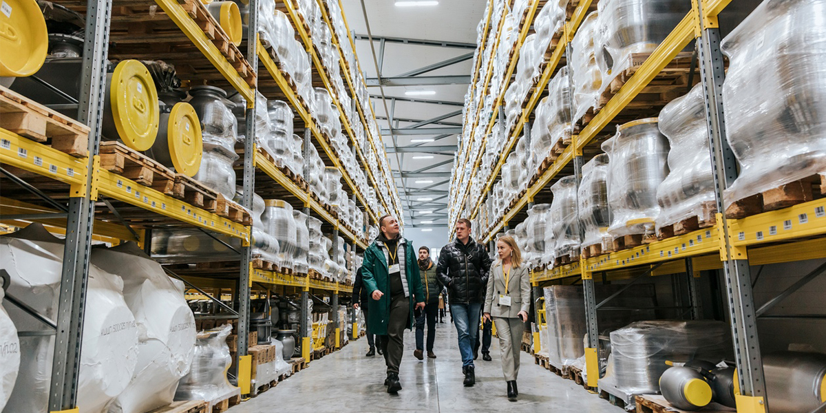
In 2018, we made a project to introduce a WMS system at the warehouse of the LD Trading House company in Chelyabinsk. Introduced the product “1C-Logistics: Warehouse Management 3” for 20 jobs: WMS operators, storekeepers, forklift drivers. Warehouse average of about 4 thousand m2, the number of cells 5000 and the number of SKU 4500. The warehouse stores ball valves of their own production in different sizes from 1 kg to 400 kg. Inventories are stored in the context of batches due to the need to select goods according to FIFO and the "in-line" specifics of product placement (explanation below).
When designing automation schemes for warehouse processes, we were faced with the existing problem of non-optimal storage of stocks. Stacking and storage of cranes has, as we have already said, “in-line” specifics. That is, the products in the cell are stacked in rows one on top of the other, and the ability to put a piece on a piece is often absent (they simply fall, and the weight is not small). Because of this, it turns out that only one nomenclature of one batch can be in one piece storage unit;
Products arrive at the warehouse daily and each arrival is a separate batch. In total, as a result of 1 month of warehouse operation, 30 separate lots are created, despite the fact that each should be stored in a separate cell. The goods are often selected not in whole pallets, but in pieces, and as a result, in the area of piece selection in many cells, the following picture is observed: in a cell with a volume of more than 1 m3 there are several pieces of cranes that occupy less than 5-10% of the cell volume (see Fig. . one).
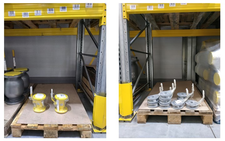
Fig 1. Photo of several pieces in a cell
On the face of the suboptimal use of storage capacity. To imagine the scale of the disaster, I can cite the figures: on average there are between 100 and 300 cells of such cells with a "scanty" residue in different periods of the warehouse’s operation. Since the warehouse is relatively small, in the warehouse loading seasons this factor becomes a “bottleneck” and greatly inhibits the warehouse processes of acceptance and shipment.
Idea of solving a problem
The idea came up: to bring the balances with the closest dates to one single lot and place such balances with a unified batch compactly together in one cell, or in several if there isn’t enough space in one to accommodate the total number of balances. An example of such a “compression” is shown in Figure 2.
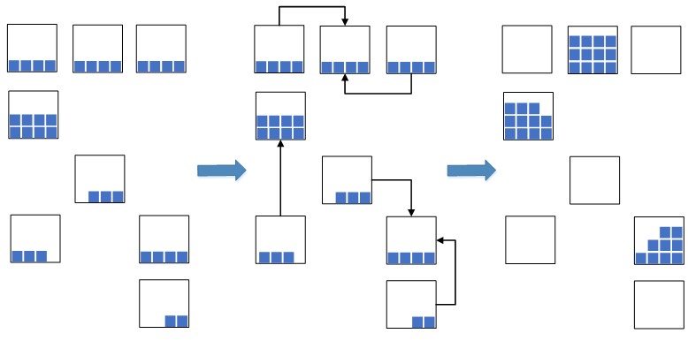
Fig. 2. Cell compression scheme
This allows you to significantly reduce the occupied warehouse space, which will be used for the newly placed goods. In the situation of overloading warehouse capacities, such a measure is extremely necessary, otherwise there may simply not be enough free space for placing new goods, which will lead to a stopper in the warehouse processes of placement and replenishment and, as a result, a stopper for acceptance and shipment. Previously, before the WMS system was implemented, such an operation was performed manually, which was not effective, since the process of finding suitable residues in the cells was quite long. Now, with the introduction of WMS systems, they decided to automate the process, speed it up and make it intelligent.
The process of solving this problem is divided into 2 stages:
- at the first stage, we find groups of parties that are close in date for compression (to this dedication task, the previous article );
- at the second stage, for each group of batches we calculate the most compact placement of product residues in cells.
In the current article, we will stop at the second stage of the algorithm.
Overview of existing solutions
Before proceeding to the description of the algorithms developed by us, it is worthwhile to conduct a brief review of the WMS systems already existing on the market, which implement similar optimal compression functionality.
First of all, it is necessary to note the product “1C: Enterprise 8. WMS Logistics. Warehouse Management 4 ”, which is owned and replicated by 1C and belongs to the fourth generation of WMS systems developed by AXELOT. In this system, compression functionality is declared, which is designed to combine disparate product residues in one common cell. It is worth mentioning that the compression functionality in such a system also includes other features, for example, correcting the placement of goods in cells according to their ABC classes, but we will not dwell on them.
If you analyze the code of the system "1C: Enterprise 8. WMS Logistics. Warehouse Management 4 ”(which is open in this part of the functional), then we can conclude the following. The residual compression algorithm implements a rather primitive linear logic and there can be no talk of any “optimal” compression. Naturally, he does not provide for the clustering of parties. Several clients with such a system implemented complained about the results of compression planning. For example, often in practice during compression the following situation happened: 100 pcs. it is planned to move the remaining goods from one cell to another cell, where 1 pc is lying. goods, although it is optimal in terms of time to do the opposite.
Also, the compression functionality of the residual goods in the cells is declared in many foreign WMS systems, but, unfortunately, we don’t have any real feedback on the efficiency of the algorithms (this is a trade secret), nor even more about the depth of their logic (proprietary software with closed code) we don’t have, therefore we cannot judge.
Search for a mathematical model of a problem
In order to design high-quality algorithms for solving a problem, it is first necessary to clearly formulate this problem mathematically, which we will do.
There are many cells J in which the remains of some goods. Further, such cells will be called donor cells. We denote wj volume of goods in the cell $j $.
It is important to say that only one product of one consignment, or several consignments, previously grouped together in a cluster (read the previous article ) can participate in the compression procedure, which is due to the specifics of storage and packing of goods. For different products or different batches clusters, a separate compression procedure should be launched.
There are many cells I into which residues from donor cells can potentially be placed. Such cells will be called container cells. These can be either free cells in the warehouse or donor cells from a variety of J . Always a lot J is a subset I .
For each cell i out of many I capacity limits set di measured in dm3. One dm3 is a cube with sides of 10 cm. The products stored in the warehouse are quite large, so in this case, such a discretization is enough.
The shortest distance matrix is given sij in meters between each pair of cells (i,j) where i and j belong to the sets I and J respectively.
We denote Sij "Costs" for moving goods from the cell i to cell j . We denote Di "Costs" for choosing a container i to move residues from other cells into it. How exactly and in what units of measurement will the values be calculated Sij and Di we will consider further (see the preparation of input data section), now it’s enough to say that such quantities will be directly proportional to the quantities sij and di respectively.
Denote by xij a variable taking value 1 if the remainder of the cell j move to container i , and 0 otherwise. Denote by yi variable taking value 1 if container i contains the remains of the goods, and 0 otherwise.
The task is as follows : it is necessary to find so many containers I∗ and thus “attach” donor cells to cell containers to minimize function
minF= sumi inI, j inJSij cdotxij+ sumi inIDi cdotyi
under restrictions
sumj inJwj cdotxij leqdi cdotyi, for everyone i inI
In total, in the course of computing the solution to the problem, we strive to:
- firstly, save storage capacity;
- secondly, save storekeepers time.
The last restriction means that we cannot move goods to a container that we have not selected, and therefore we have not “incurred costs” for choosing it. This restriction also means that the volume of goods transported from cells to the container should not exceed the capacity of the container. By the solution of the problem we mean a lot of containers I∗ and methods for attaching donor cells to containers.
This formulation of the optimization problem is not new, and has been studied by many mathematicians since the beginning of the 80s of the last century. In foreign literature, there are 2 optimization problems with a suitable mathematical model: Single-Source Capacitated Facility Location Problem and Multi-Source Capacitated Facility Location Problem (we will discuss the differences between the tasks below). It is worth saying that in the mathematical literature the statements of these two optimization problems are formulated in terms of locating enterprises on the ground, hence the name “Facility Location”. For the most part, this is a tribute to tradition, since for the first time the need for solving such combinatorial problems came from the field of logistics, for the most part, the military-industrial growth in the 50s of the last century. In terms of the location of enterprises, such tasks are formulated as follows:
- There are a finite number of cities where it is potentially possible to locate manufacturing enterprises (hereinafter manufacturing cities). For each manufacturing city, the costs for opening an enterprise in it, as well as a restriction on the production capacity of the enterprise opened in it, are set.
- There are a finite number of cities where clients are actually located (hereinafter referred to as client cities). For each such client city, the volume of demand for products is set. For simplicity, we assume that the product that enterprises produce and consume customers is one.
- For each pair, the manufacturer city and the client city, the value of transport costs for the delivery of the required volume of products from the manufacturer to the client is set.
It is required to find in which cities to open enterprises and how to attach customers to such enterprises in order to:
- The total cost of opening enterprises and transportation costs were minimal;
- The volume of customer demand attached to any open enterprise did not exceed the production capacities of this enterprise.
Now it is worth mentioning the only difference in these two classical problems:
- Single-Source Capacitated Facility Location Problem - the client is supplied only from one open enterprise;
- Multi-Source Capacitated Facility Location Problem - a client can be supplied from several open enterprises at the same time.
Such a difference between the two problems at first glance is insignificant, but, in fact, leads to a completely different combinatorial structure of such problems and, as a result, to completely different algorithms for solving them. The differences between the tasks are shown in the figure below.
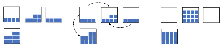
Fig. 3. a) Multi-Source Capacitated Facility Location Problem
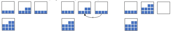
Fig. 3. b) Single-Source Capacitated Facility Location Problem
Both tasks NP are difficult, that is, there is no exact algorithm that would solve such a problem in polynomial time from the size of the input data. In simpler words, all the exact algorithms for solving the problem will work exponentially, although perhaps faster than a complete search of the options face to face. Since the task NP is difficult, then we will consider only approximate heuristics, that is, algorithms that will stably calculate solutions that are very close to optimal and will work quickly enough. If there is interest in such a task, then here you can find a good review in Russian.
If we shift to the terminology of our problem of optimal compression of goods in cells, then:
- client cities are donor cells J with the remains of the goods,
- manufacturing cities - container cells I into which residues from other cells are supposed to be placed,
- transport costs - time costs Sij storekeeper to move the volume of goods from the donor cell j to the container cell i ;
- the cost of opening an enterprise - the cost of choosing a container Di equal to the volume of the container cell i multiplied by a certain coefficient of economy of free volumes (the value of the coefficient is always> 1) (see the preparation of input data section).
After the analogy with the well-known classical deliveries of the problem has been drawn, it is necessary to answer the important question on which the choice of the solution algorithm architecture depends: the movement of residues from the donor cell is possible only in one and only one container (Single-Source), or the movement of residues is possible into multiple container cells (Multi-Source)?
It should be noted that in practice both formulations of the problem have a place to be. We give all the pros and cons for each such statement below:
| Task option | Pluses of option | Cons of option |
|---|---|---|
| Single source | Operations of moving goods calculated according to this option of the task:
| |
| Multi source | Compressions calculated according to this variant of the task are usually more compact by 10-15% compared to compressions calculated according to the “Single-Source” variant. But also note that the smaller the number of residues in the donor cells, the smaller the difference in compactness. | Operations of moving goods calculated according to this option of the task:
|
Since the number of pluses for the Single-Source option is greater, and also taking into account the fact that the smaller the number of residuals in the donor cells, the smaller the difference in the degree of compression compactness calculated for both versions of the problem, our choice fell on the Single- Source
It is worth saying that the solution of the Multi-Source option also takes place. There are a large number of effective algorithms for its solution, most of which boil down to solving a number of transport problems. There are also not only efficient algorithms, but also elegant ones, for example, here.
Input preparation
Before proceeding to the analysis and development of an algorithm for solving the problem, it is necessary to determine what data and in what form we will submit it to the input. There are no problems with the volumes of goods left in the donor cells and the capacity of the container cells, since this is trivial - such values will be measured in m3, but with the costs of using the container container and the cost matrix for moving, it is not so simple!
First, consider the calculation of the cost of moving goods from a donor cell to a container cell. First of all, it is necessary to determine in what units of measurement we will calculate the cost of moving. The two most obvious options are meters and seconds. In "clean" meters, the cost of moving is pointless. We show this by example. Let the cell A located on the first tier, cell To removed 30 meters and is located on the second tier:
- Moving out A at B more costly than moving from B at A , since it is easier to lower down from the second tier (1.5-2 meters from the floor) than to raise to the second, although the distance will be the same;
- Move 1 pc. goods from the cell A at B It will be easier than moving 10 pcs. of the same product, although the distance will be the same.
Movement costs are best taken into account in seconds, since this allows you to take into account the difference in tiers and the difference in the quantity of goods transported. To account for the costs of movement in seconds, we must decompose the operation of movement to elementary components and take measurements of time for each elementary component.
Let from the cell j moves Nj PC. goods to container i . Let be Srun - the average speed of the employee in the warehouse, measured in m / s. Let be Sget and Sput - average speeds of a single execution of operations to take and put, respectively, for the volume of goods equal to 4 dm3 (the average volume that an employee in the warehouse takes for 1 time during operations). Let be Hget and Hput the height of the cells from which the operations are performed take and put accordingly. For example, the average height of the first tier (floor) is 1 m, the second tier is 2 m, etc. Then the formula for calculating the total time to complete the move operation Tij following:
Tij= left(Nj cdot fracwj4 right) cdotSget cdotHget+sij cdotSrun+ left(Nj cdot fracwj4 right) cdotSput cdotHput.
Table 2 shows the statistics of the execution time of each elementary operation, collected by the warehouse staff, taking into account the specifics of the stored goods.
| the name of the operation | Designation | Average value |
|---|---|---|
| The average speed of the employee in the warehouse | Srun | 1,5 m / s |
| Put the average speed of one operation (for a volume of goods 4 dm3) | Sput | 2.4 sec |
With the method of calculating the cost of moving decided. Now you need to figure out how to calculate the cost of choosing a container cell . Here, everything is much, much more complicated than with the cost of moving, because:
- firstly, the costs should be directly dependent on the volume of the cell - it is better to put the same volume of residues transferred from donor cells into a container of a smaller volume than into a large container, provided that such a volume fits completely in both containers . So, by minimizing the total cost of choosing containers, we strive to save “scarce” free storage capacity in the area of the selection zone for the subsequent operations of placing goods in cells. Figure 4 shows the options for moving residues to large and small containers and the consequences of such options for moving during subsequent warehouse operations.
- -, , , , - , .
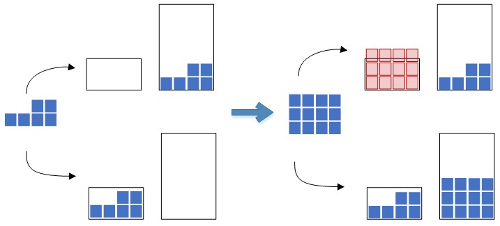
Fig. 4. Options for moving residues into containers of different capacities.
Figure 4 shows in red the volume of residues that no longer fits in the container at the second stage of the placement of subsequent goods.
The following requirements for calculated solutions to the problem will help you connect cubic meters of container costs with seconds of moving costs:
- It is necessary that the residues from the donor cell be moved to the container cell in any case, if this reduces the total number of container cells in which the goods are located.
- It is necessary to maintain a balance between the volumes of containers and the time spent on moving: for example, if the new solution to the problem compares with a large gain in the volume and the time loss is small, then you need to choose a new one.
Let's start with the last requirement. In order to specify the ambiguous word “balance”, we conducted a survey of warehouse employees in order to find out the following. Let there be a cell container volumed 0 , in which the movement of the remnants of goods from donor cells is assigned and the total time of such movement isT 0 . Suppose there are several alternative options for placing the same quantity of goods from the same donor cells in other containers, where each placement has its own ratings d 1 where d 1 < d 0 and T 1 where T 1 > T 0 .
The question is: what is the minimum gain in volume d 0 - d 1 is acceptable, for a given value of time lossT 1 - T 0 ?Let us illustrate with an example. Initially, the residues were supposed to be placed in a container of 1000 dm3 (1 m3) volume and the travel time was 70 seconds. There is an option of placing residues in another container with a volume of 500 dm3 and a time of 130 seconds. Question: are we ready to spend an additional 60 seconds of the storekeeper’s time on moving in order to save 500 dm3 of free volume? Based on a survey of warehouse employees, the following chart was compiled.
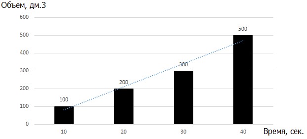
Fig. 5. Diagram of the dependence of the minimum allowable volume saving on the increase in the difference in the operation time.
That is, if the additional time costs are 40 seconds, then we are ready to spend them only when the gain in volume is at least 500 dm3. Despite the fact that a slight nonlinearity is observed in the dependence, for simplicity of further calculations, we assume that the dependence between the quantities is linear and is described by the inequality
d 0 - d 110 ≥T1-T0
In the figure below, we consider the following methods of placing goods in containers.
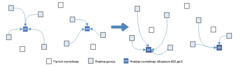
Fig. 6. Option (a): 2 containers, total volume 400 dm3, total time 150 sec.
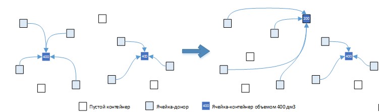
Fig. 6. Option (b): 2 containers, total volume 600 dm3, total time 190 sec.
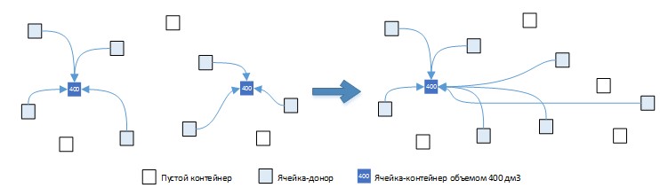
Fig. 6. Option (s): 1 container, total volume 400 dm3, total time 200 sec.
Option (a) of the choice of containers is more preferable than the original option, since the inequality holds: (800-400) / 10> = 150-120, which implies 40> = 30. Option (b) is less preferable than the original option , since the inequality does not hold: (800-600) / 10> = 190-150, which implies 20> = 40. But option (c) does not fit into this logic! Let's consider this option in more detail. On the one hand, the inequality (800-400) / 10> = 200-120, which means that the inequality 40> = 80 is not fulfilled, which means that the gain in volume is not worth such a big loss in time.
But on the other hand, in this option (c), we not only reduce the total occupied volume, but also reduce the number of occupied cells, which is the first of two important requirements for the calculated solutions to the problems listed above. Obviously, in order for this requirement to begin to be fulfilled, it is necessary to add some positive constant to the left side of the inequalityC o n s t , and such a constant needs to be added only when the number of containers decreases. Recall thaty i is a variable equal to 1 when the containeri is selected, and 0 when the containeri not selected. DenoteI 0 is the set of containers in the original solution andI 1 - many containers in the new solution. In general terms, the new inequality will look like this:
∑ i∈ I 0 d i10 +Const⋅∑ i∈ I 0 yi-(∑ i∈ I 1 d i10 +Const⋅∑ i∈ I 1 yi)≥T1-T0
Transforming the inequality above, we obtain
∑ i∈ I 0 d i10 +Const⋅∑ i∈ I 0 yi+T0≥∑ i∈ I 1 d i10 +Const⋅∑ i∈ I 1 yi+T1
Based on this, we have a formula for calculating the total cost F k some solution to the problem:
F k =∑ i∈ I k d i10 +Const⋅∑ i∈ I k yi+Tk.
But now the question arises : what value should such a constant have?C o n s t ?Obviously, its value must be large enough so that the first requirement for the solution of the problem is always satisfied. You can of course take a constant value equal to 10 3 or 10 6 , but I would like to avoid such "magic numbers". If we consider the specifics of performing warehouse operations, we can calculate several well-founded numerical estimates of the magnitude of such a constant.
Let be S m a x - the maximum distance between the cells of the warehouse of one zone ABC, equal in our case to 100 m. Letd m a x - the maximum volume of the container cell in the warehouse, equal in our case to 1000 dm3. The first way to calculate the value
C o n s t . Consider the situation when there are 2 containers on the first tier in which the goods are already physically located, that is, they themselves are donor cells, and the cost of moving the goods to the same cells is naturally 0. It is necessary to find such a constant value C o n s t , in which it would be advantageous to always move residues from container 1 to container 2. Substituting valuesS m a x and d m a x to the inequality above, we obtain:
d m a x10 +Const≥Smax⋅srun+d m a x4 (sget+sput),
what follows
C o n s t ≥ S m a x ⋅ s r u n + d m a x ( s g e t + s p u t4 -110 ).
Substituting the values of the average execution time of elementary operations in the formula above, we obtain
C o n s t ≥ 100 ⋅ 1 , 5 + 1000 ( 910 )→Const≥1050.
The second way to calculate the value C o n s t . Consider a situation where there is N donor cells from which it is planned to move the goods into container 1. DenoteS 1 j is the distance from the donor cellj to container 1. There is also container 2, in which there are already goods, and the volume of which allows you to accommodate the remainingN cells. For simplicity, we will assume that the volume of goods transported from donor cells to containers is the same and equald m a x / N . It is required to find such a constant value C o n s t at which the placement of all residues fromN cells in container 2 would always be more profitable than placing them in different containers:
2 ⋅ d m a x10+2⋅Const+N(S1j⋅srun+dmax4⋅N(sget+sput))≥dmax10 +Const+N⋅(Smax⋅srun+ d m a x4 ⋅ N (sget+sput)).
Transforming the inequality we get
d m a x10 +Const+N⋅S1j⋅srun≥N⋅Smax⋅srun→Const≥N⋅srun(Smax-S1j)-d m a x10 .
In order to "strengthen" the value of the quantity C o n s t , we assume thatS 1 j = 0. The average number of cells that are usually involved in the process of compressing residual stock is 10. Substituting the known values of the quantities, we have the following constant value
C o n s t ≥ 10 ⋅ 1 , 5 ⋅ 100 - 100010 →Const≥1400.
We take the largest value calculated for each option, this will be the value of C o n s t for given warehouse parameters. Now for completeness, we write the formula for calculating total costsF k for some feasible solutionk :
F k =∑ i∈ I k d i10 +1400⋅∑ i∈ I k yi+Tk.
Now, after all the titanic efforts to convert the input data, we can say that all the input data is converted to the desired form and is ready for use in the optimization algorithm.
Conclusion
As practice shows, the complexity and importance of the preparation and conversion of the input data for the algorithm is often underestimated. In this article, we specifically paid a lot of attention to this stage in order to show that only qualitatively and wisely prepared input data can make the decisions calculated by the algorithm really valuable for the client. Yes, there were many conclusions of the formulas, but we warned you before the kat :)
In the next article, we will finally come to what the 2 previous publications thought about - the discrete optimization algorithm.
The article was prepared by
Roman Shangin, Programmer, Project Department,
First Bit Company, Chelyabinsk
All Articles