Inverse problems of affine transformations or about one beautiful formula
In this article I will talk about one unusual formula that allows you to look at a new angle on affine transformations, and especially on inverse problems that arise in connection with these transformations. I will call inverse problems that require computing the inverse matrix: finding the transformation by points, solving a system of linear equations, transforming coordinates when changing the basis, etc. I’ll make a reservation right away that there will be no fundamental discoveries in the article, nor a reduction in algorithmic complexity — I will just show a symmetrical and easily remembered formula with which you can solve unexpectedly many running problems. For lovers of mathematical rigor, there is a more formal presentation here [1] (oriented to students) and a small task book here [2] .
The affine transformation is usually defined by the matrix A and translation vector and acts on the vector argument by the formula
However, you can do without vect if you use the augmented matrix and uniform coordinates for the argument (as is well known to OpenGL users). However, it turns out, besides these forms of writing, you can also use the determinant of a special matrix, which contains both the coordinates of the argument and the parameters that determine the transformation. The fact is that the determinant has the property of linearity over the elements of any row or column, and this allows it to be used to represent affine transformations. Here, in fact, how to express the effect of the affine transformation on an arbitrary vector vecx :

Do not rush to run away in horror - firstly, a transformation is written here that acts on spaces of arbitrary dimension (there are so many things from here), and secondly, although the formula looks cumbersome, it is simply remembered and used. To start, I will highlight the logically related elements with frames and color

So we see that the action of any affine transformation mathcalA per vector can be represented as the ratio of two determinants, with the vector argument entering only the top, and the bottom is just a constant that depends only on the parameters.
Blue highlighted vector vecx Is an argument, the vector on which the affine transformation acts mathcalA . Hereinafter, subscripts denote the component of the vector. In the upper matrix of the components vecx occupy almost the entire first column, except for them in this column only zero (top) and one (bottom). All other elements in the matrix are parameter vectors (they are numbered by the superscript, taken in brackets so as not to confuse with the degree) and units in the last row. Parameters distinguish from the set of all affine transformations what we need. The convenience and beauty of the formula is that the meaning of these parameters is very simple: they define an affine transformation that translates vectors vecx(i) at vecX(i) . Therefore vectors vecx(1), dots, vecx(n+1) , we will call “input” (they are surrounded by rectangles in the matrix) - each of them is written component-wise in its own column, and a unit is added from below. “Output” parameters are written from above (highlighted in red) vecX1, dots, vecXn+1 , but now not componentwise, but as a whole entity.
If someone is surprised by such a record, then remember the vector product
where there was a very similar structure and the first line in the same way was occupied by vectors. Moreover, it is not necessary that the dimensions of the vectors vecX(i) and vecx(i) coincided. All determinants are considered as usual and allow the usual "tricks", for example, you can add another column to any column.
With the bottom matrix, everything is extremely simple - it is obtained from the top by deleting the first row and first column. The disadvantage of (1) is that you have to consider the determinants, however, if you transfer this routine task to a computer, it turns out that a person will only have to fill in the matrix correctly with numbers from his task. At the same time, using one formula, you can solve quite a few common practice problems:
Under the influence of an unknown affine transformation, three points on the plane passed to the other three points. Find this affine transformation.
 For definiteness, let our entry points

and the result of the transformation

Find the affine transformation mathcalA .
In fact, this problem can be solved in different ways: with the help of a system of linear equations, barycentric coordinates ... but we will go our own way. I think that by the notation used, you can guess what I'm getting at: we take equation (1) for the dimension n=2 and substitute vecx(i) as input parameters, and vecX(i) - as a weekend
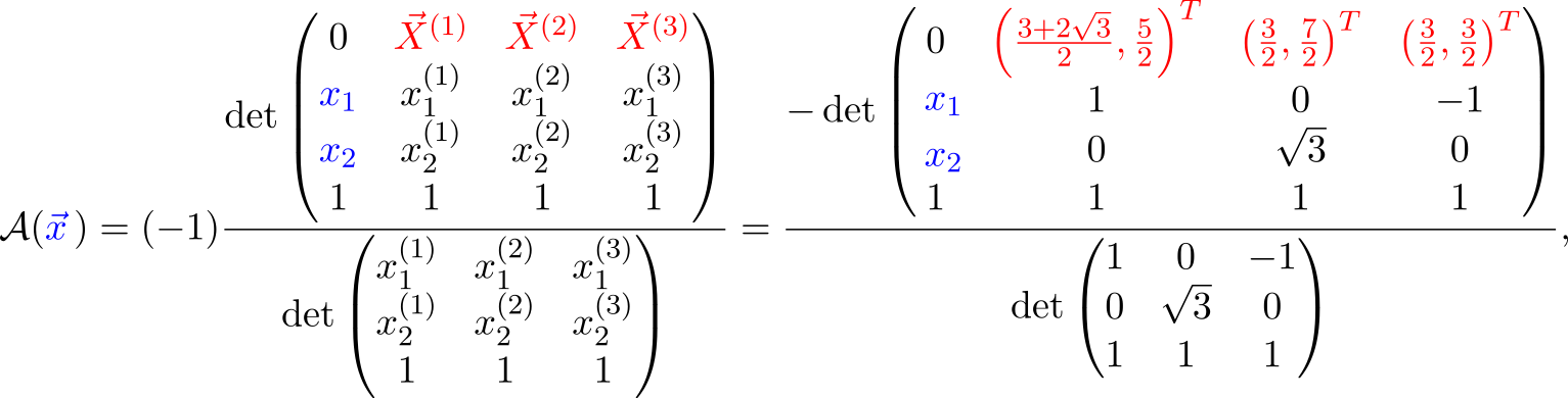
and then it remains only to calculate the determinants

A trained eye will easily detect a turn on 30 circ and broadcast on ((3+ sqrt3)/2,2) mathsfT .
Input and output vectors can have different dimensions - the formula is applicable for affine transformations acting on spaces of any dimension. However, there should be enough input points and they should not “stick together”: if the affine transformation acts from n -dimensional space - points must form a non-degenerate simplex from n+1 points. If this condition is not met, then it is impossible to unambiguously restore the transformation (by any method at all, not only this) - the formula will warn about this by zero in the denominator.
Often you need to find a transformation between two pictures (for calculating the position of the camera, for example). If we have some reliable special points (features) in these images, or you just don’t want to start right away with ranzaks and fight with outlayers, then this formula can be used.
Another example is texturing . Cutting a triangle from a texture and pulling it onto a triangle somewhere on a plane or in space is a typical task for applying the affine transformation to points from a texture space, translating them into the space where the models live. And quite often it’s easy for us to indicate which points on the texture correspond to the vertices of the model’s triangle, but to establish where the non-corner points go may require some thought. With the same formula, it’s enough to simply insert the numbers into the correct cells and there will be such beauty.

From what I had to face personally: the neural network gives the coordinates of the marker corners and we want to “complement reality” with a virtual object located on the marker.
Obviously, when moving the marker, the object must repeat all its movements. And here the formula (1) is very useful - it will help us move the object after the marker.
Or another example: you need to program the rotation of various objects on the stage using the gizmo tool. To do this, we must be able to rotate the selected model around three axes parallel to the coordinate axes and passing through the center of the object. The picture shows the case of rotation of the model around an axis parallel to Oz .

Ultimately, it all comes down to the two-dimensional problem of rotation around an arbitrary point. Let's even solve it for some simple case, say, turning on 90 circ counterclockwise around (a;b) (the general case is solved the same way, I just don’t want to clutter the calculations with sines and cosines). Of course, you can go the way of the samurai and multiply three matrices (translation of the rotation point to zero, actually rotation and translation back), or you can find the coordinates of any three points before and after rotation and use the formula. The first point is easy - we already know that (a;b) goes into itself. Let's look at the point one to the right, for it is true (a+1;b) mapsto(a;b+1) . Well, one more one below, it is obvious that (a;b−1) mapsto(a+1;b) . Then everything is simple

We decompose the upper determinant (1) along the first line according to the Laplace rule. It is clear that as a result we get some weighted sum of vectors vecX(i) . It turns out that the coefficients in this sum are the barycentric coordinates of the argument vecx in relation to the simplex given vecx(i) (for proofs see [1] ). If we are interested only in the barycentric coordinates of a point, we can cheat and fill the first line with unit orts - after calculating the determinants we get a vector whose components coincide with the barycentric coordinates vecx . Graphically, such a transformation mathcalB translating a point into the space of its barycentric coordinates will look as follows

Let's try this "recipe" in practice. Task: find the barycentric coordinates of a point with respect to a given triangle. Let it be a point for definiteness (2,2) mathsfT , and take the vertices of a triangle

The point is small - take (1) for n=2 , correctly place the task data there and calculate the determinants

Here is the solution: barycentric coordinates (2,2) mathsfT with respect to a given triangle there is 0.6 , 0.3 and 0.1 . In programming, the calculation of barycentric coordinates often arises in the context of checking whether a point is inside a simplex (then all barycentric coordinates are more than zero and less than unity), as well as for various interpolations, which we will discuss now.
Note that formula (1) has a pleasant duality: if we expand the determinant in the first column, we get the standard notation for the affine function, and if on the first line we get the affine combination of output vectors.
So, we found that the affine transformation weights the output vectors with coefficients equal to the barycentric coordinates of the argument. It is natural to use this property for multilinear interpolation.
For example, let's calculate the standard GL ‑ th “hello world” - a colored triangle. Of course, OpenGL can perfectly interpolate colors and also does this using barycentric coordinates , but today we will do it ourselves.
Task: at the vertices of the triangle the colors are set, to interpolate the colors inside the triangle. For definiteness, let the vertices of our triangle have coordinates

We assign them colors: yellow, cyan and magenta

Number triples are the RGB components of a color. Take (1) and correctly arrange the input data

Here are the components mathcalC(x;y) indicate how to paint a point (x,y) in terms of RGB. Let's see what happened.
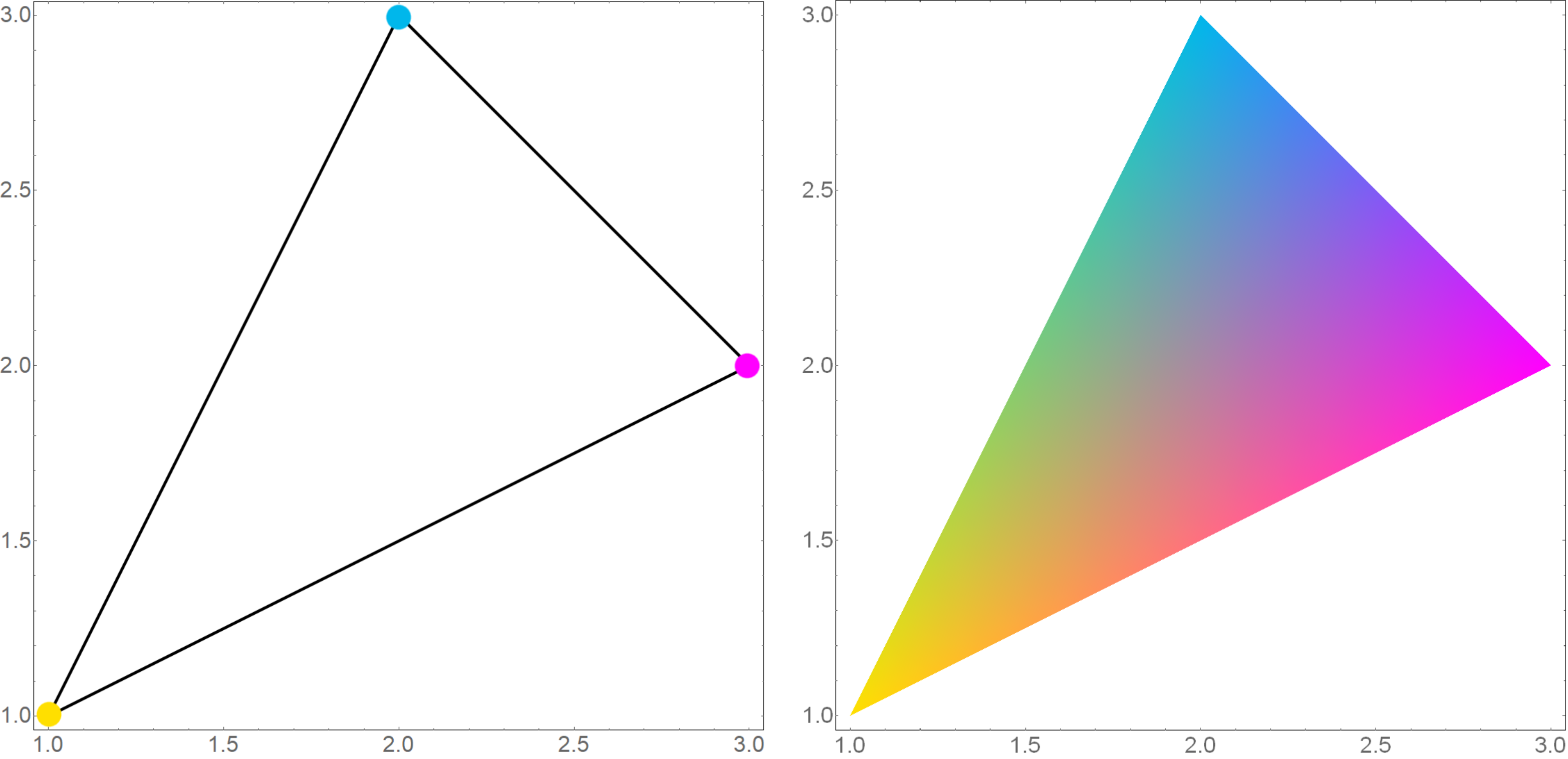
We can say that we just made an affine transformation of the two-dimensional space of a picture into a three-dimensional space of colors (RGB).
We can put a variety of meanings in the vectors that we interpolate, including those that can be normal vectors. Moreover, this is exactly what Phong shading is done for, only after interpolation the vectors need to be normalized. Why this interpolation is needed is well illustrated by the following image (taken from Wikipedia commons.wikimedia.org/w/index.php?curid=1556366 ).
I don’t think it’s worth making calculations anymore - all the details are discussed in [2] , but I will show a picture with the result.

The vectors on it are not single and for use in Phong shading, they must first be normalized, and, for clarity, they are directed in very different directions, which is rarely the case in practice.
Consider another unusual example of the application of the affine transformation.
Three points are given

We find the equation of the plane passing through them in the form z=z(x,y) . And we will do this with the help of affine transformations: after all, it is known that they translate planes in planes. To start, we design all the points on the plane Xy that is easy. And now we will establish an affine transformation that translates the projections of points to the original three-dimensional points

and which "picks up" along with the points and the entire plane Xy so much so that after the transformation it will go through the points of interest to us.
As usual, we only have to distribute the numbers among the elements of the matrices

Rewrite the last expression in the usual form

and draw what happened.
Despite the practical importance of affine transformations, one often has to deal with linear ones. Of course, linear transformations are a special case of affine transformations, leaving a point in place vec0 . This allows us to simplify the formula a little (after all, one of the columns will consist of almost only zeros and you can expand the determinant by it)

As you can see, the last row with units and one column is missing from the formula. This result is completely consistent with our ideas that to specify a linear transformation, it suffices to indicate its effect on n linearly independent elements.
Let's solve the problem to see how everything works. Problem: it is known that under the action of some linear transformation

We find this linear transformation.
We take a simplified formula and put the correct numbers in the right places:

Done!
Recall that the linear transformation matrix

contains images of unit vectors in its columns:

So, acting as a matrix on the unit vectors, we get its columns. But what about the inverse transformation (let's say it exists)? It does everything the other way around:

Wait a minute, because we just found the images of three points under the influence of a linear transformation - enough to restore the transformation itself!

Where vece1=(1;0;0) mathsfT , vece2=(0;1;0) mathsfT and vece3=(0;0;1) mathsfT .
We will not limit ourselves to three-dimensional space and rewrite the previous formula in a more general form

As you can see, we need to assign to the matrix on the left a column with the components of the vector argument, on top - a line with coordinate vectors, and then it’s only the ability to take determinants.
Let's try the given method in practice. Task: invert the matrix

We use (2) for n=3

It is immediately clear that

From school, we are faced with equations of the form

If the matrix hatA non-degenerate, then the solution can be written as

Hmm ... is it not in the previous section that I saw the same expression, but instead b was another letter? We will use it.

This is none other than Cramer’s rule . This can be easily verified by expanding the determinant on the first line: calculation xi just assumes that we cross out the column with vecei , and with it i Matrix column hatA . Now if you rearrange the column b instead of the remote one, then we just get the rule "insert column b in place i Th column and find the determinant. " And yes, all is well with the signs: alone pm we generate when expanding along the line, and others when rearranging - as a result, they cancel each other out.
Looking at the resulting equation, you can notice its similarity with the equation for finding barycentric coordinates: the solution of a system of linear equations is finding the barycentric coordinates of a point vecb in relation to a simplex, one of the vertices of which vec0 , and the rest are defined by the columns of the matrix hatA .
We solve the system of linear equations

In matrix form, it looks like this

We use the resulting formula

where does the answer come from x=1/25 , y = 14 / 25 and z = 2 / 5 .
Suppose that we have chosen a new basis (moved to a different coordinate system). It is known that the new coordinates of the vectors are expressed through the old linearly. Therefore, it is not surprising that we can use our tools to change the basis. How to do this, I will show with an example.
So, let us move from the standard basis \ {\ vec {e} _x, \ vec {e} _y \} to a basis consisting of vectors

In the old basis, a vector is specified v e c x = ( 3 , 4 ) m a t h s f T . Find the coordinates of this vector in a new basis. In the new coordinate system, the vectors of the new basis will become orts and will have coordinates

hereinafter, the strokes near the columns mean that the coordinates in them refer to a new basis. It’s easy to guess that a linear transformation that translates

also converts the coordinates of our vector as needed. It remains only to apply the formula

The solution of the problem in the usual way requires matrix inversion (which, however, also mainly consists of calculating determinants) and multiplication

We just packed these steps into one formula.
The effectiveness of the formula in solving inverse problems is explained by the following equality (the proof is in [1] )

Thus, the formula hides in itself the inverse matrix and multiplication by another matrix in addition. This expression is the standard solution to the problem of finding a linear transformation by points.Note that making the second matrix in the product identity, we get just the inverse matrix. With its help, a system of linear equations and the problems that can be reduced to it are solved: finding barycentric coordinates, interpolation by Lagrange polynomials, etc. However, the representation in the form of a product of two matrices does not allow us to get the very “two glances” associated with the expansion on the first row and on the first column.
Let me remind you that Lagrange interpolation is finding the least polynomial passing through points( a 0 ; b 0 ) , ( a 1 ; b 1 ) , ... , ( a n ; b n ) . Not that it was a common task in programmer practice, but let's look at it anyway.
The fact is that the polynomial

can be considered as a linear transformation that displays the vector ( x n ; x n - 1 ; ... ; 1 ) T at R . So the point interpolation problem ( a 0 ; b 0 ) , ( a 1 ; b 1 ) , ... , ( a n ; b n ) reduces to finding a linear transformation such that

and we are able to do this. Substitute the correct letters in the correct cells and get the formula

The proof that this will be the Lagrange polynomial (and not someone else) can be found in [1] . By the way, the expression in the denominator is Vandermonde's identifier. Knowing this and expanding the determinant in the numerator along the first line, we arrive at a more familiar formula for the Lagrange polynomial.
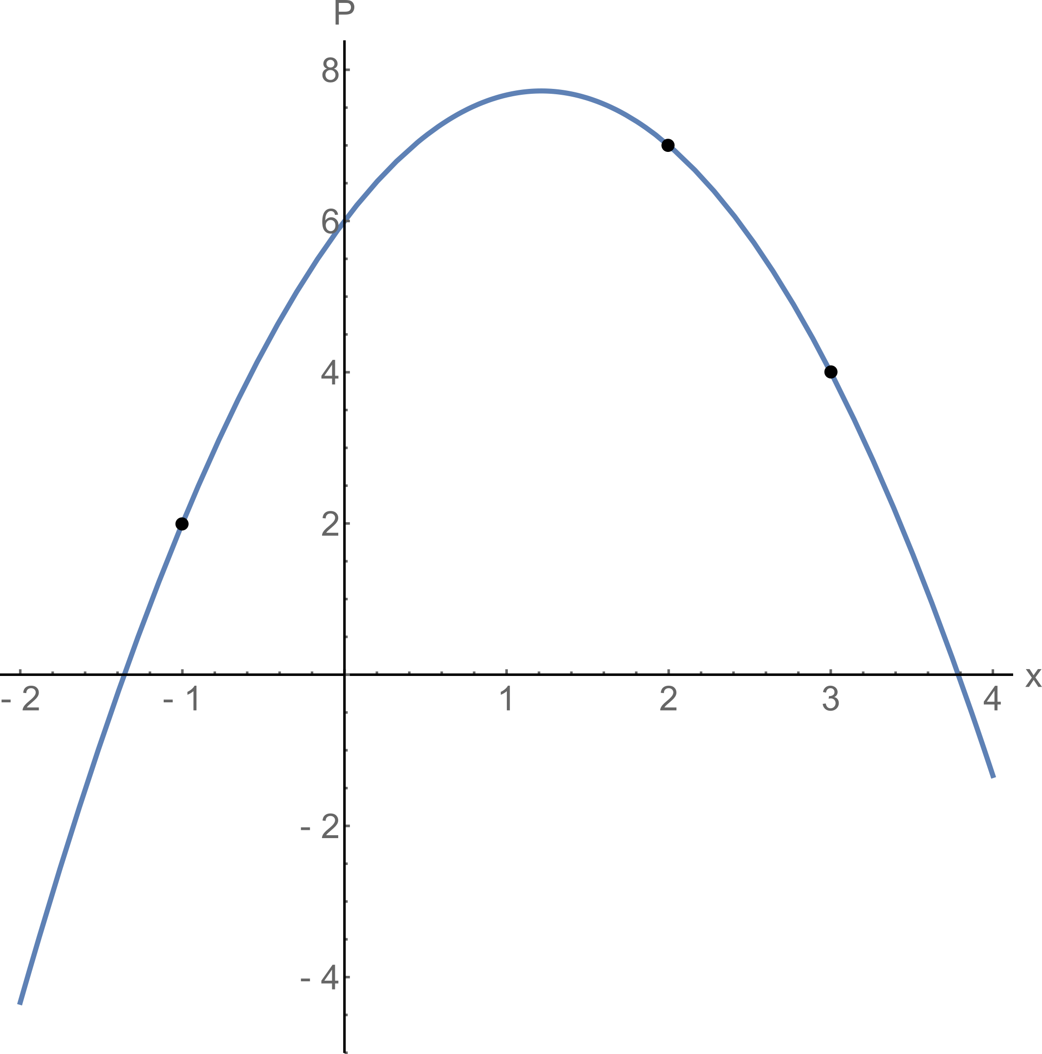
Is it difficult to use? Let's try the forces on the problem: find the Lagrange polynomial passing through the points( - 1 ; 2 ) , ( 3 ; 4 ) and ( 2 ; 7 ) .
Substitute these points in the formula

On the chart, everything will look like this.
Having laid out the upper determinant in the first row and first column, we look at the Lagrange polynomial from two different sides. In the first case, we get the classic formula from Wikipedia, and in the second, we write the polynomial in the form of the sum of monomialsα i x i where

And now we can relatively easily prove rather complicated statements. For example, in [2] it was proved in one line that the sum of the basic Lagrange polynomials is equal to one and that the Lagrange polynomial interpolating( a 0 ; a n + 1 0 ) , ... , ( a n ; a n + 1 n ) , has a value of zero( - 1 ) n a 0 ⋅ ⋯ ⋅ a n . Well, not a single Lagrange - a similar approach can be applied to interpolation by sines-cosines or some other functions.
Thanks to everyone who read to the end. In this article, we solved standard problems using one non-standard formula. I liked it because, firstly, it shows that affine (linear) transformations, barycentric coordinates, interpolation, and even Lagrange polynomials are closely related. After all, when solutions to problems are written in the same way, the thought of their affinity arises by itself. Secondly, most of the time we simply arranged the input data in the correct cells without additional transformations.
The tasks that we considered can also be solved by quite familiar methods. However, for problems of small dimension or educational tasks, the formula may be useful. In addition, she seems beautiful to me.
[ 1] Beginner's guide to mapping simplexes affinely
[ 2] Workbook on mapping simplexes affinely
The affine transformation is usually defined by the matrix A and translation vector
and acts on the vector argument by the formula
mathcalA( vecx)= hatA vecx+ vect.
However, you can do without vect if you use the augmented matrix and uniform coordinates for the argument (as is well known to OpenGL users). However, it turns out, besides these forms of writing, you can also use the determinant of a special matrix, which contains both the coordinates of the argument and the parameters that determine the transformation. The fact is that the determinant has the property of linearity over the elements of any row or column, and this allows it to be used to represent affine transformations. Here, in fact, how to express the effect of the affine transformation on an arbitrary vector vecx :
Do not rush to run away in horror - firstly, a transformation is written here that acts on spaces of arbitrary dimension (there are so many things from here), and secondly, although the formula looks cumbersome, it is simply remembered and used. To start, I will highlight the logically related elements with frames and color
So we see that the action of any affine transformation mathcalA per vector can be represented as the ratio of two determinants, with the vector argument entering only the top, and the bottom is just a constant that depends only on the parameters.
Blue highlighted vector vecx Is an argument, the vector on which the affine transformation acts mathcalA . Hereinafter, subscripts denote the component of the vector. In the upper matrix of the components vecx occupy almost the entire first column, except for them in this column only zero (top) and one (bottom). All other elements in the matrix are parameter vectors (they are numbered by the superscript, taken in brackets so as not to confuse with the degree) and units in the last row. Parameters distinguish from the set of all affine transformations what we need. The convenience and beauty of the formula is that the meaning of these parameters is very simple: they define an affine transformation that translates vectors vecx(i) at vecX(i) . Therefore vectors vecx(1), dots, vecx(n+1) , we will call “input” (they are surrounded by rectangles in the matrix) - each of them is written component-wise in its own column, and a unit is added from below. “Output” parameters are written from above (highlighted in red) vecX1, dots, vecXn+1 , but now not componentwise, but as a whole entity.
If someone is surprised by such a record, then remember the vector product
[\ vec {a} \ times \ vec {b}] = \ det \ begin {pmatrix} \ vec {e} _1 & \ vec {e} _2 & \ vec {e} _3 \\ a_1 & a_2 & a_3 \\ b_1 & b_2 & b_3 \\ \ end {pmatrix},
[\ vec {a} \ times \ vec {b}] = \ det \ begin {pmatrix} \ vec {e} _1 & \ vec {e} _2 & \ vec {e} _3 \\ a_1 & a_2 & a_3 \ \ b_1 & b_2 & b_3 \\ \ end {pmatrix},
where there was a very similar structure and the first line in the same way was occupied by vectors. Moreover, it is not necessary that the dimensions of the vectors vecX(i) and vecx(i) coincided. All determinants are considered as usual and allow the usual "tricks", for example, you can add another column to any column.
With the bottom matrix, everything is extremely simple - it is obtained from the top by deleting the first row and first column. The disadvantage of (1) is that you have to consider the determinants, however, if you transfer this routine task to a computer, it turns out that a person will only have to fill in the matrix correctly with numbers from his task. At the same time, using one formula, you can solve quite a few common practice problems:
- finding an affine transformation by points;
- calculation of barycentric coordinates;
- multilinear interpolation;
- linear transformation problems (without translation):
Three-point affine transformation on a plane
Under the influence of an unknown affine transformation, three points on the plane passed to the other three points. Find this affine transformation.
For definiteness, let our entry points
and the result of the transformation
Find the affine transformation mathcalA .
In fact, this problem can be solved in different ways: with the help of a system of linear equations, barycentric coordinates ... but we will go our own way. I think that by the notation used, you can guess what I'm getting at: we take equation (1) for the dimension n=2 and substitute vecx(i) as input parameters, and vecX(i) - as a weekend
and then it remains only to calculate the determinants
A trained eye will easily detect a turn on 30 circ and broadcast on ((3+ sqrt3)/2,2) mathsfT .
When is the formula applicable?
Input and output vectors can have different dimensions - the formula is applicable for affine transformations acting on spaces of any dimension. However, there should be enough input points and they should not “stick together”: if the affine transformation acts from n -dimensional space - points must form a non-degenerate simplex from n+1 points. If this condition is not met, then it is impossible to unambiguously restore the transformation (by any method at all, not only this) - the formula will warn about this by zero in the denominator.
Why restore affine transformations to a programmer?
Often you need to find a transformation between two pictures (for calculating the position of the camera, for example). If we have some reliable special points (features) in these images, or you just don’t want to start right away with ranzaks and fight with outlayers, then this formula can be used.
Another example is texturing . Cutting a triangle from a texture and pulling it onto a triangle somewhere on a plane or in space is a typical task for applying the affine transformation to points from a texture space, translating them into the space where the models live. And quite often it’s easy for us to indicate which points on the texture correspond to the vertices of the model’s triangle, but to establish where the non-corner points go may require some thought. With the same formula, it’s enough to simply insert the numbers into the correct cells and there will be such beauty.
From what I had to face personally: the neural network gives the coordinates of the marker corners and we want to “complement reality” with a virtual object located on the marker.
Obviously, when moving the marker, the object must repeat all its movements. And here the formula (1) is very useful - it will help us move the object after the marker.
Or another example: you need to program the rotation of various objects on the stage using the gizmo tool. To do this, we must be able to rotate the selected model around three axes parallel to the coordinate axes and passing through the center of the object. The picture shows the case of rotation of the model around an axis parallel to Oz .
Ultimately, it all comes down to the two-dimensional problem of rotation around an arbitrary point. Let's even solve it for some simple case, say, turning on 90 circ counterclockwise around (a;b) (the general case is solved the same way, I just don’t want to clutter the calculations with sines and cosines). Of course, you can go the way of the samurai and multiply three matrices (translation of the rotation point to zero, actually rotation and translation back), or you can find the coordinates of any three points before and after rotation and use the formula. The first point is easy - we already know that (a;b) goes into itself. Let's look at the point one to the right, for it is true (a+1;b) mapsto(a;b+1) . Well, one more one below, it is obvious that (a;b−1) mapsto(a+1;b) . Then everything is simple
Barycentric coordinates
We decompose the upper determinant (1) along the first line according to the Laplace rule. It is clear that as a result we get some weighted sum of vectors vecX(i) . It turns out that the coefficients in this sum are the barycentric coordinates of the argument vecx in relation to the simplex given vecx(i) (for proofs see [1] ). If we are interested only in the barycentric coordinates of a point, we can cheat and fill the first line with unit orts - after calculating the determinants we get a vector whose components coincide with the barycentric coordinates vecx . Graphically, such a transformation mathcalB translating a point into the space of its barycentric coordinates will look as follows
Let's try this "recipe" in practice. Task: find the barycentric coordinates of a point with respect to a given triangle. Let it be a point for definiteness (2,2) mathsfT , and take the vertices of a triangle
The point is small - take (1) for n=2 , correctly place the task data there and calculate the determinants
Here is the solution: barycentric coordinates (2,2) mathsfT with respect to a given triangle there is 0.6 , 0.3 and 0.1 . In programming, the calculation of barycentric coordinates often arises in the context of checking whether a point is inside a simplex (then all barycentric coordinates are more than zero and less than unity), as well as for various interpolations, which we will discuss now.
Note that formula (1) has a pleasant duality: if we expand the determinant in the first column, we get the standard notation for the affine function, and if on the first line we get the affine combination of output vectors.
Multilinear interpolation
So, we found that the affine transformation weights the output vectors with coefficients equal to the barycentric coordinates of the argument. It is natural to use this property for multilinear interpolation.
Color interpolation
For example, let's calculate the standard GL ‑ th “hello world” - a colored triangle. Of course, OpenGL can perfectly interpolate colors and also does this using barycentric coordinates , but today we will do it ourselves.
Task: at the vertices of the triangle the colors are set, to interpolate the colors inside the triangle. For definiteness, let the vertices of our triangle have coordinates
We assign them colors: yellow, cyan and magenta
Number triples are the RGB components of a color. Take (1) and correctly arrange the input data
Here are the components mathcalC(x;y) indicate how to paint a point (x,y) in terms of RGB. Let's see what happened.
We can say that we just made an affine transformation of the two-dimensional space of a picture into a three-dimensional space of colors (RGB).
Normal Interpolation (Phong Shading)
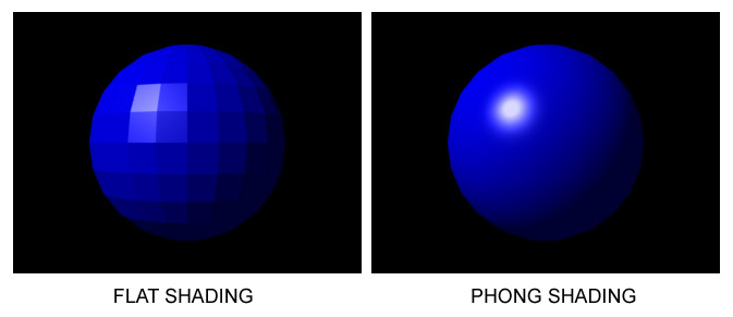
We can put a variety of meanings in the vectors that we interpolate, including those that can be normal vectors. Moreover, this is exactly what Phong shading is done for, only after interpolation the vectors need to be normalized. Why this interpolation is needed is well illustrated by the following image (taken from Wikipedia commons.wikimedia.org/w/index.php?curid=1556366 ).
I don’t think it’s worth making calculations anymore - all the details are discussed in [2] , but I will show a picture with the result.
The vectors on it are not single and for use in Phong shading, they must first be normalized, and, for clarity, they are directed in very different directions, which is rarely the case in practice.
Find plane z=z(x,y) at three points
Consider another unusual example of the application of the affine transformation.
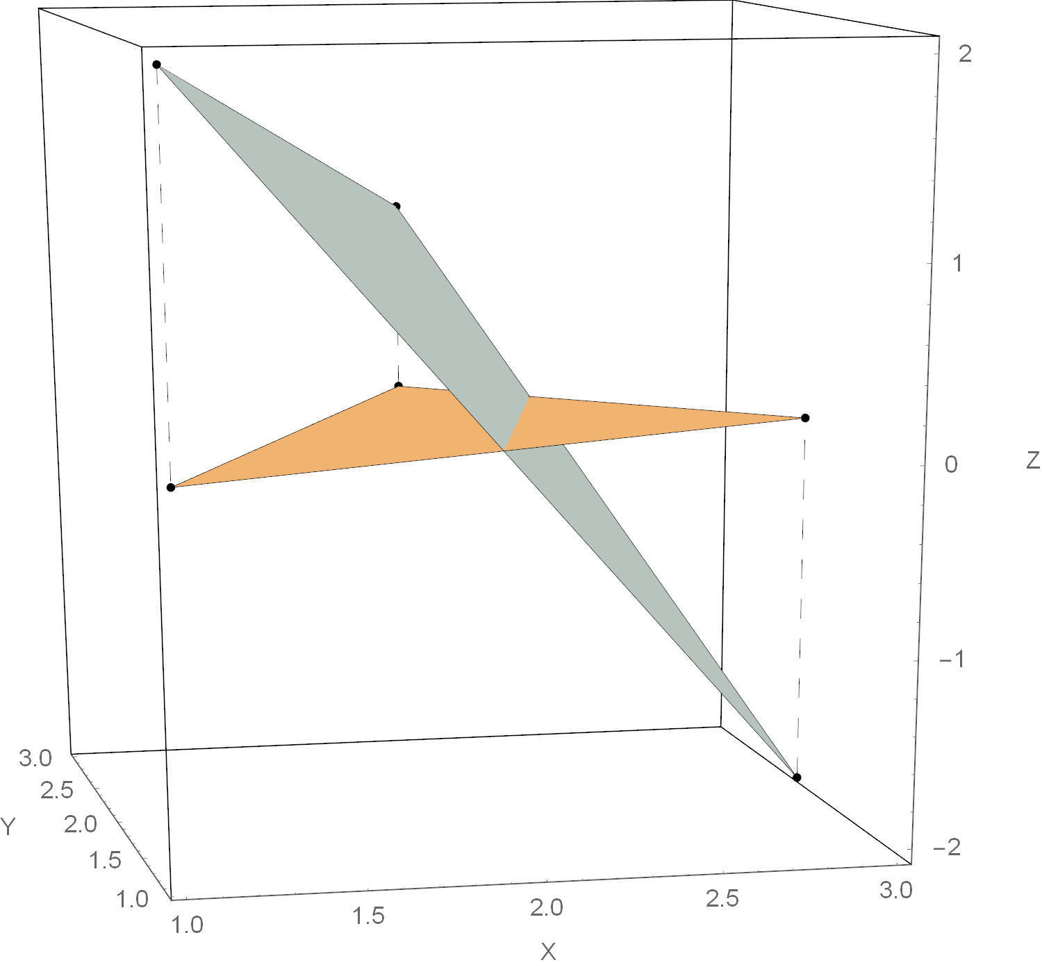
Three points are given
We find the equation of the plane passing through them in the form z=z(x,y) . And we will do this with the help of affine transformations: after all, it is known that they translate planes in planes. To start, we design all the points on the plane Xy that is easy. And now we will establish an affine transformation that translates the projections of points to the original three-dimensional points
and which "picks up" along with the points and the entire plane Xy so much so that after the transformation it will go through the points of interest to us.
As usual, we only have to distribute the numbers among the elements of the matrices
Rewrite the last expression in the usual form
and draw what happened.
Linear transformations
Despite the practical importance of affine transformations, one often has to deal with linear ones. Of course, linear transformations are a special case of affine transformations, leaving a point in place vec0 . This allows us to simplify the formula a little (after all, one of the columns will consist of almost only zeros and you can expand the determinant by it)
As you can see, the last row with units and one column is missing from the formula. This result is completely consistent with our ideas that to specify a linear transformation, it suffices to indicate its effect on n linearly independent elements.
Three-point linear transformation
Let's solve the problem to see how everything works. Problem: it is known that under the action of some linear transformation
We find this linear transformation.
We take a simplified formula and put the correct numbers in the right places:
Done!
Finding the inverse transform
Recall that the linear transformation matrix
contains images of unit vectors in its columns:
So, acting as a matrix on the unit vectors, we get its columns. But what about the inverse transformation (let's say it exists)? It does everything the other way around:
Wait a minute, because we just found the images of three points under the influence of a linear transformation - enough to restore the transformation itself!
Where vece1=(1;0;0) mathsfT , vece2=(0;1;0) mathsfT and vece3=(0;0;1) mathsfT .
We will not limit ourselves to three-dimensional space and rewrite the previous formula in a more general form
As you can see, we need to assign to the matrix on the left a column with the components of the vector argument, on top - a line with coordinate vectors, and then it’s only the ability to take determinants.
Inverse Transformation Problem
Let's try the given method in practice. Task: invert the matrix
We use (2) for n=3
It is immediately clear that
Cramer rule in one formula
From school, we are faced with equations of the form
If the matrix hatA non-degenerate, then the solution can be written as
Hmm ... is it not in the previous section that I saw the same expression, but instead b was another letter? We will use it.
This is none other than Cramer’s rule . This can be easily verified by expanding the determinant on the first line: calculation xi just assumes that we cross out the column with vecei , and with it i Matrix column hatA . Now if you rearrange the column b instead of the remote one, then we just get the rule "insert column b in place i Th column and find the determinant. " And yes, all is well with the signs: alone pm we generate when expanding along the line, and others when rearranging - as a result, they cancel each other out.
Looking at the resulting equation, you can notice its similarity with the equation for finding barycentric coordinates: the solution of a system of linear equations is finding the barycentric coordinates of a point vecb in relation to a simplex, one of the vertices of which vec0 , and the rest are defined by the columns of the matrix hatA .
Solution of a system of linear equations
We solve the system of linear equations
In matrix form, it looks like this
We use the resulting formula
where does the answer come from x=1/25 , y = 14 / 25 and z = 2 / 5 .
Transformation of vector coordinates when changing the basis
Suppose that we have chosen a new basis (moved to a different coordinate system). It is known that the new coordinates of the vectors are expressed through the old linearly. Therefore, it is not surprising that we can use our tools to change the basis. How to do this, I will show with an example.
So, let us move from the standard basis \ {\ vec {e} _x, \ vec {e} _y \} to a basis consisting of vectors
In the old basis, a vector is specified v e c x = ( 3 , 4 ) m a t h s f T . Find the coordinates of this vector in a new basis. In the new coordinate system, the vectors of the new basis will become orts and will have coordinates
hereinafter, the strokes near the columns mean that the coordinates in them refer to a new basis. It’s easy to guess that a linear transformation that translates
also converts the coordinates of our vector as needed. It remains only to apply the formula
The solution of the problem in the usual way requires matrix inversion (which, however, also mainly consists of calculating determinants) and multiplication
We just packed these steps into one formula.
Why does the formula work for inverse problems?
The effectiveness of the formula in solving inverse problems is explained by the following equality (the proof is in [1] )
Thus, the formula hides in itself the inverse matrix and multiplication by another matrix in addition. This expression is the standard solution to the problem of finding a linear transformation by points.Note that making the second matrix in the product identity, we get just the inverse matrix. With its help, a system of linear equations and the problems that can be reduced to it are solved: finding barycentric coordinates, interpolation by Lagrange polynomials, etc. However, the representation in the form of a product of two matrices does not allow us to get the very “two glances” associated with the expansion on the first row and on the first column.
Lagrange interpolation and its properties
Let me remind you that Lagrange interpolation is finding the least polynomial passing through points( a 0 ; b 0 ) , ( a 1 ; b 1 ) , ... , ( a n ; b n ) . Not that it was a common task in programmer practice, but let's look at it anyway.
How are polynomials and linear transforms related?
The fact is that the polynomial
can be considered as a linear transformation that displays the vector ( x n ; x n - 1 ; ... ; 1 ) T at R . So the point interpolation problem ( a 0 ; b 0 ) , ( a 1 ; b 1 ) , ... , ( a n ; b n ) reduces to finding a linear transformation such that
and we are able to do this. Substitute the correct letters in the correct cells and get the formula
The proof that this will be the Lagrange polynomial (and not someone else) can be found in [1] . By the way, the expression in the denominator is Vandermonde's identifier. Knowing this and expanding the determinant in the numerator along the first line, we arrive at a more familiar formula for the Lagrange polynomial.
Problem on the Lagrange polynomial
Is it difficult to use? Let's try the forces on the problem: find the Lagrange polynomial passing through the points( - 1 ; 2 ) , ( 3 ; 4 ) and ( 2 ; 7 ) .
Substitute these points in the formula
On the chart, everything will look like this.
Properties of the Lagrange polynomial
Having laid out the upper determinant in the first row and first column, we look at the Lagrange polynomial from two different sides. In the first case, we get the classic formula from Wikipedia, and in the second, we write the polynomial in the form of the sum of monomialsα i x i where
And now we can relatively easily prove rather complicated statements. For example, in [2] it was proved in one line that the sum of the basic Lagrange polynomials is equal to one and that the Lagrange polynomial interpolating( a 0 ; a n + 1 0 ) , ... , ( a n ; a n + 1 n ) , has a value of zero( - 1 ) n a 0 ⋅ ⋯ ⋅ a n . Well, not a single Lagrange - a similar approach can be applied to interpolation by sines-cosines or some other functions.
Conclusion
Thanks to everyone who read to the end. In this article, we solved standard problems using one non-standard formula. I liked it because, firstly, it shows that affine (linear) transformations, barycentric coordinates, interpolation, and even Lagrange polynomials are closely related. After all, when solutions to problems are written in the same way, the thought of their affinity arises by itself. Secondly, most of the time we simply arranged the input data in the correct cells without additional transformations.
The tasks that we considered can also be solved by quite familiar methods. However, for problems of small dimension or educational tasks, the formula may be useful. In addition, she seems beautiful to me.
Bibliography
[ 1] Beginner's guide to mapping simplexes affinely
[ 2] Workbook on mapping simplexes affinely
All Articles