Automatically detect emotions in text conversations using neural networks
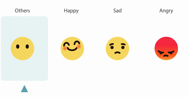
One of the main tasks of interactive systems is not only to provide the information the user needs, but also to generate as many human answers as possible. And recognition of the interlocutor’s emotions is no longer just a cool feature, it is a vital necessity. In this article, we will look at the architecture of a recurrent neural network for determining emotions in text conversations , which took part in the SemEval-2019 Task 3 “EmoContext” , the annual competition in computer linguistics. The task was to classify emotions (“happy”, “sad”, “angry” and “others”) in a conversation of three remarks, in which a chat bot and a person participated.
In the first part of the article we will consider the task set in EmoContext and the data provided by the organizers. In the second and third parts, we analyze the preliminary processing of the text and the ways of vector representation of words. In the fourth part, we describe the LSTM architecture that we used in the competition. The code is written in Python using the Keras library.
1. Training data
The track “EmoContext” at SemEval-2019 was dedicated to the definition of emotions in text conversations, taking into account the context of correspondence. The context in this case is several consecutive remarks of dialogue participants. There are two participants in the conversation: an anonymous user (he owns the first and third replica) and a chat bot Ruuh (he owns the second replica). Based on three replicas, it is necessary to determine what emotion the user experienced when writing an answer to the chatbot (Table 1). In total, the markup of the dataset contained four emotions: “happy”, “sad”, “angry” or “others” (Table 1). A detailed description is presented here: ( Chatterjee et al., 2019 ).
Table 1. Examples from the EmoContext dataset ( Chatterjee et al., 2019 )
| User (Stage-1) | Interactive Robot (Stage-1) | User (Stage-2) | True class |
|---|---|---|---|
| I just qualified for the Nabard internship | WOOT! That's great news. Congratulations! | I started crying | Happiness |
| How dare you to slap my child | If you spoil my car, I will do that to you too | Just try to do that once | Anger |
| I was hurt by u more | You didn't mean it. | say u love me | Sadness |
| I will do night. | Alright. Keep me in loop. | Not giving WhatsApp no. | Other |
During the competition, the organizers provided several data sets. The training dataset (Train) consisted of 30,160 manually marked texts. In these texts there were approximately 5000 objects belonging to the classes “happy”, “sad” and “angry”, as well as 15000 texts from the class “others” (Table 2).
The organizers also provided data sets for development (Dev) and testing (Test), in which, unlike the training dataset, the distribution by class of emotions corresponded to real life: about 4% for each of the classes “happy”, “sad” and “ angry ", and the rest is the class" others ". Data provided by Microsoft, you can download it in the official group on LinkedIn .
Table 2. Distribution of emotion class labels in the dataset ( Chatterjee et al., 2019 ).
| Datacet | Happiness | Sadness | Anger | Other | Total |
|---|---|---|---|---|---|
| Training
| 14.07%
| 18.11%
| 18.26%
| 49.56%
| 30 160
|
| For development
| 5.15%
| 4.54%
| 5.45%
| 84.86%
| 2755
|
| Test
| 5.16%
| 4.54%
| 5.41%
| 84.90%
| 5509
|
| Remote
| 33.33%
| 33.33%
| 33.33%
| 0%
| 900 thousand
|
In addition to this data, we collected 900 thousand English-language messages from Twitter to create a Distant dataset (300 thousand tweets for each emotion). In creating it, we followed the strategy of Go et al. (2009), in the framework of which messages were simply associated with the presence of words related to emotions, such as #angry, #annoyed, #happy, #sad, #surprised and so on. The list of terms is based on the terms from the SemEval-2018 AIT DISC ( Duppada et al., 2018 ).
The main quality metric in the EmoContext competition is the average F1 measure for the three classes of emotions, that is, for the classes “happy”, “sad” and “angry”.
def preprocessData(dataFilePath, mode): conversations = [] labels = [] with io.open(dataFilePath, encoding="utf8") as finput: finput.readline() for line in finput: line = line.strip().split('\t') for i in range(1, 4): line[i] = tokenize(line[i]) if mode == "train": labels.append(emotion2label[line[4]]) conv = line[1:4] conversations.append(conv) if mode == "train": return np.array(conversations), np.array(labels) else: return np.array(conversations) texts_train, labels_train = preprocessData('./starterkitdata/train.txt', mode="train") texts_dev, labels_dev = preprocessData('./starterkitdata/dev.txt', mode="train") texts_test, labels_test = preprocessData('./starterkitdata/test.txt', mode="train")
2. Text pre-processing
Before training, we pre-processed the texts using the Ekphrasis tool (Baziotis et al., 2017). It helps to correct spelling, normalize words, segment, and also determine which tokens should be dropped, normalized or annotated using special tags. At the pre-processing stage, we did the following:
- URLs and mail, date and time, nicknames, percentages, currencies and numbers were replaced with corresponding tags.
- Repeating, censored, elongated uppercase terms we accompanied with appropriate labels.
- Elongated words have been automatically corrected.
In addition, Emphasis contains a tokenizer that can identify most emojis, emoticons and complex expressions, as well as dates, times, currencies and acronyms.
Table 3. Examples of text preprocessing.
| Source text | Pre-processed text |
|---|---|
I FEEL YOU ... I'm breaking into million pieces  | <allcaps> i feel you </allcaps>. <repeated> i am breaking into million pieces |
| tired and I missed you too :‑( | tired and i missed you too <sad> |
| you should liiiiiiisten to this: www.youtube.com/watch?v=99myH1orbs4 | you should listen <elongated> to this: <url> |
| My apartment takes care of it. My rent is around $ 650. | my apartment takes care of it. my rent is around <money>. |
from ekphrasis.classes.preprocessor import TextPreProcessor from ekphrasis.classes.tokenizer import SocialTokenizer from ekphrasis.dicts.emoticons import emoticons import numpy as np import re import io label2emotion = {0: "others", 1: "happy", 2: "sad", 3: "angry"} emotion2label = {"others": 0, "happy": 1, "sad": 2, "angry": 3} emoticons_additional = { '(^・^)': '<happy>', ':‑c': '<sad>', '=‑d': '<happy>', ":'‑)": '<happy>', ':‑d': '<laugh>', ':‑(': '<sad>', ';‑)': '<happy>', ':‑)': '<happy>', ':\\/': '<sad>', 'd=<': '<annoyed>', ':‑/': '<annoyed>', ';‑]': '<happy>', '(^ ^)': '<happy>', 'angru': 'angry', "d‑':": '<annoyed>', ":'‑(": '<sad>', ":‑[": '<annoyed>', '( ? )': '<happy>', 'x‑d': '<laugh>', } text_processor = TextPreProcessor( # terms that will be normalized normalize=['url', 'email', 'percent', 'money', 'phone', 'user', 'time', 'url', 'date', 'number'], # terms that will be annotated annotate={"hashtag", "allcaps", "elongated", "repeated", 'emphasis', 'censored'}, fix_html=True, # fix HTML tokens # corpus from which the word statistics are going to be used # for word segmentation segmenter="twitter", # corpus from which the word statistics are going to be used # for spell correction corrector="twitter", unpack_hashtags=True, # perform word segmentation on hashtags unpack_contractions=True, # Unpack contractions (can't -> can not) spell_correct_elong=True, # spell correction for elongated words # select a tokenizer. You can use SocialTokenizer, or pass your own # the tokenizer, should take as input a string and return a list of tokens tokenizer=SocialTokenizer(lowercase=True).tokenize, # list of dictionaries, for replacing tokens extracted from the text, # with other expressions. You can pass more than one dictionaries. dicts=[emoticons, emoticons_additional] ) def tokenize(text): text = " ".join(text_processor.pre_process_doc(text)) return text
3. Vector representation of words
Vector representation has become an integral part of most approaches to the creation of NLP-systems using deep learning. To determine the most appropriate vector mapping models, we tried Word2Vec ( Mikolov et al., 2013 ), GloVe ( Pennington et al., 2014 ) and FastText ( Joulin et al., 2017 ), as well as pre-trained DataStories vectors ( Baziotis et al. ., 2017 ). Word2Vec finds relationships between words by assuming that semantically related words are found in similar contexts. Word2Vec tries to predict the target word (CBOW architecture) or context (Skip-Gram architecture), that is, minimize the loss function, and GloVe calculates word vectors, reducing the dimension of the adjacency matrix. The logic of FastText is similar to the logic of Word2Vec, except that it uses symbolic n-grams to build word vectors, and as a result, it can solve the problem of unknown words.
For all the mentioned models, we use the default training parameters provided by the authors. We trained a simple LSTM model (dim = 64) based on each of these vector representations and compared the classification efficiency using cross-validation. The best result in F1 measures was shown by pre-trained DataStories vectors.
To enrich the selected vector mapping with the emotional coloring of words, we decided to fine-tune the vectors using the automatically labeled Distant dataset ( Deriu et al., 2017 ). We used the Distant dataset to train a simple LSTM network to classify “evil”, “sad” and “happy” messages. The embedding layer was frozen during the first iteration of training in order to avoid strong changes in the weights of vectors, and for the next five iterations the layer was thawed. After training, the “delayed” vectors were saved for later use in the neural network, as well as shared .
def getEmbeddings(file): embeddingsIndex = {} dim = 0 with io.open(file, encoding="utf8") as f: for line in f: values = line.split() word = values[0] embeddingVector = np.asarray(values[1:], dtype='float32') embeddingsIndex[word] = embeddingVector dim = len(embeddingVector) return embeddingsIndex, dim def getEmbeddingMatrix(wordIndex, embeddings, dim): embeddingMatrix = np.zeros((len(wordIndex) + 1, dim)) for word, i in wordIndex.items(): embeddingMatrix[i] = embeddings.get(word) return embeddingMatrix from keras.preprocessing.text import Tokenizer embeddings, dim = getEmbeddings('emosense.300d.txt') tokenizer = Tokenizer(filters='') tokenizer.fit_on_texts([' '.join(list(embeddings.keys()))]) wordIndex = tokenizer.word_index print("Found %s unique tokens." % len(wordIndex)) embeddings_matrix = getEmbeddingMatrix(wordIndex, embeddings, dim)
4. Neural network architecture
Recurrent Neural Networks (RNNs) are a family of neural networks that specialize in processing a series of events. Unlike traditional neural networks, RNNs are designed to work with sequences using internal balances. For this, the computational graph RNN contains cycles that reflect the influence of previous information from the sequence of events on the current one. LSTM neural networks (Long Short-Term Memory) were introduced as an extension of RNN in 1997 ( Hochreiter and Schmidhuber, 1997 ). LSTM recurrence cells are connected in such a way as to avoid problems with the explosion and attenuation of gradients. Traditional LSTMs only preserve past information as they process the sequence in one direction. Bidirectional LSTMs operating in both directions combine the output of two hidden LSTM layers that transmit information in opposite directions - one in the course of time and the other against - thereby simultaneously receiving data from past and future states ( Schuster and Paliwal, 1997 ).

Figure 1: Reduced version of the architecture. The LSTM module uses the same weights for the first and third stages.
A simplified representation of the described approach is shown in Figure 1. The architecture of the neural network consists of an embedding layer and two bidirectional LTSM modules (dim = 64). The first LTSM module analyzes the words of the first user (i.e., the first and third replica of the conversation), and the second module analyzes the words of the second user (second replica). At the first stage, the words of each user using pre-trained vector representations are fed into the corresponding bidirectional LTSM module. Then the resulting three feature maps are combined into a flat feature vector, and then transferred to a fully connected hidden layer (dim = 30), which analyzes the interactions between the extracted features. Finally, these characteristics are processed in the output layer using the softmax activation function to determine the final class label. To reduce overfitting, after layers of the vector representation, regularization layers with Gaussian noise were added, and dropout layers were added to each LTSM module (p = 0.2) and a hidden fully connected layer (p = 0.1) ( Srivastava et al., 2014 )
from keras.layers import Input, Dense, Embedding, Concatenate, Activation, \ Dropout, LSTM, Bidirectional, GlobalMaxPooling1D, GaussianNoise from keras.models import Model def buildModel(embeddings_matrix, sequence_length, lstm_dim, hidden_layer_dim, num_classes, noise=0.1, dropout_lstm=0.2, dropout=0.2): turn1_input = Input(shape=(sequence_length,), dtype='int32') turn2_input = Input(shape=(sequence_length,), dtype='int32') turn3_input = Input(shape=(sequence_length,), dtype='int32') embedding_dim = embeddings_matrix.shape[1] embeddingLayer = Embedding(embeddings_matrix.shape[0], embedding_dim, weights=[embeddings_matrix], input_length=sequence_length, trainable=False) turn1_branch = embeddingLayer(turn1_input) turn2_branch = embeddingLayer(turn2_input) turn3_branch = embeddingLayer(turn3_input) turn1_branch = GaussianNoise(noise, input_shape=(None, sequence_length, embedding_dim))(turn1_branch) turn2_branch = GaussianNoise(noise, input_shape=(None, sequence_length, embedding_dim))(turn2_branch) turn3_branch = GaussianNoise(noise, input_shape=(None, sequence_length, embedding_dim))(turn3_branch) lstm1 = Bidirectional(LSTM(lstm_dim, dropout=dropout_lstm)) lstm2 = Bidirectional(LSTM(lstm_dim, dropout=dropout_lstm)) turn1_branch = lstm1(turn1_branch) turn2_branch = lstm2(turn2_branch) turn3_branch = lstm1(turn3_branch) x = Concatenate(axis=-1)([turn1_branch, turn2_branch, turn3_branch]) x = Dropout(dropout)(x) x = Dense(hidden_layer_dim, activation='relu')(x) output = Dense(num_classes, activation='softmax')(x) model = Model(inputs=[turn1_input, turn2_input, turn3_input], outputs=output) model.compile(loss='categorical_crossentropy', optimizer='adam', metrics=['acc']) return model model = buildModel(embeddings_matrix, MAX_SEQUENCE_LENGTH, lstm_dim=64, hidden_layer_dim=30, num_classes=4)
5. Results
In the search for the optimal architecture, we experimented not only with the number of neurons in the layers, activation functions and regularization parameters, but also with the architecture of the neural network itself. This is described in more detail in the original work .
The architecture described in the previous section showed the best results when training on the Train dataset and validation on the Dev dataset, so it was used in the final stage of the competition. At the last test dataset, the model showed a micro-averaged F1 measure of 72.59%, and the maximum achieved result among all participants was 79.59%. Nevertheless, our result was much higher than the base value of 58.68%, set by the organizers.
The source code for the model and vector representation of words is available on GitHub.
The full version of the article and work with the task description are on the ACL Anthology website.
The training dataset can be downloaded from the official LinkedIn group.
Citation:
@inproceedings{smetanin-2019-emosense, title = "{E}mo{S}ense at {S}em{E}val-2019 Task 3: Bidirectional {LSTM} Network for Contextual Emotion Detection in Textual Conversations", author = "Smetanin, Sergey", booktitle = "Proceedings of the 13th International Workshop on Semantic Evaluation", year = "2019", address = "Minneapolis, Minnesota, USA", publisher = "Association for Computational Linguistics", url = "https://www.aclweb.org/anthology/S19-2034", pages = "210--214", }
All Articles