Statistics at the service of the business. Multiple Experiment Calculation Methodology
Good day!
As promised in the previous article , today we will continue our discussion of the methodologies used in A / B testing and consider methods for evaluating the results of multiple experiments. We will see that the methodologies are quite simple, and mathematical statistics are not so scary, and the main basis of all is analytical thinking and common sense. However, I would like to say a few words about what kind of business problems help to solve rigorous mathematical methods, whether you need them at this stage of your company’s development, and what pros and cons exist in Big analytics.
In any startup flying at insane speeds, decisions are made with the same speed, and the effect of a newly launched product feature is usually so financially tangible that additional evidence is not required.
However, at a certain point in time, the company reaches such a scale and audience reach that, firstly, the task of expanding and searching for new sources of financial growth in the market due to its limited resource intensity becomes more and more difficult, and, secondly, losses from wrong decisions become critical - because without a preliminary study, without taking into account the statistical error of its results, the killer feature, presented to a product with an audience of several million DAUs, can lead to a user outflow second, improve the bounce-rate and stupendous losses in product sales that are only multiplying in the long run. In such a situation, the quick-and-dirty approach of fast analytics ceases to be useful and should give way to the approach of thoughtful and slow, thorough data analysis.
In addition, in large services that set themselves the tasks of strategic long-term planning and competent distribution of financial investments between parts of the product, conducting short- and long-term experiments is one of the most important tasks. However, for the quality and reliability of the decision made, one often has to pay with speed.
It should be noted that despite the heading of this paragraph, the scope of A / B tests extends much further beyond the boundaries of product analytics: this is the analysis of the quality of forecast models to assess future return on investment, and the study of the effectiveness of financial investments in various parts of the product and its advertising channels promotions, distribution analytics, LTV forecasting, financial modeling, quality assessment of scoring''s implemented ML-models, ranking and much more.
There are two types of experiments: those conducted with independent samples that are as consistent as possible with respect to each other at the same moment in time and those conducted with dependent samples or with the same group, but at different times.
A typical A / B product experiment that studies the effect of a new feature on key metrics refers to experiments with independent samples. Investigation of the influence of a factor during which it is impossible to distinguish between groups that interacted with the source of impact and those that did not interact, and therefore, it is possible to evaluate the impact only on the basis of metrics before and after, refers to the study with dependent samples. An example of such a study is the analysis of the results of an advertising company on TV. Another option for conducting an experiment with dependent samples may be a study in the format of pairwise comparisons of elements between groups, in which each element of the control sample is assigned an element of the experimental sample.
There are also A / A experiments and inverse experiments. These topics are quite interesting, but we will not consider them in detail in the framework of this article.
In addition, experiments can be carried out both in A / B format and in the format of multiple comparisons, as stated in the title of the article. Since the typical methodologies for calculating the A / B experiment were considered earlier , in this article we will talk about the methodologies for calculating multiple experiments and recommendations on the boundaries of their use for solving business problems.
As mentioned above, sometimes in practice, multiple comparisons are made
It should be noted that each new split group added to the study reduces its accuracy, reduces the representativeness of the sample, and also increases the likelihood of an error of the first kind: for simultaneously conducted experiments the level of statistical significance is at the accepted alpha level for one experiment of 5%.
Why do multiple experiments, if they reduce the accuracy of the results of our study?
The first reason may be the desire of the business as soon as possible and cheaper to get an answer, which decision should be made if there are several options, saving the time and cost of developing and implementing the experiment.
The second reason may be testing combinations - the simplest example: the user is offered a different mutual arrangement of the two elements on the landing page.
In addition, one of the tasks of conducting a multiple test, although controversial in terms of accuracy of assessment for a number of reasons, may be the desire to conduct A / A / B - conducting parallel studies of A / A and A / B in order to verify the reliability of the results and eliminate the probability of a false-positive result (recall the famous article by David Kodavi about A / A ).
Today we will consider a typical and widespread task of introducing a new feature in order to increase the company's revenue by increasing the number of targeted monetized actions. At the entrance, we have three groups of users who were offered 3 different delivery options with the offer to click on the call button for an ad.
To test multiple hypotheses, approaches from the theory of analysis of variance, otherwise called ANOVA, are used. Moreover, in most cases, calculation and verification of the group probability of an error of the first kind FWER occurs.
The essence of FWER is quite simple: we evaluate the likelihood of false-positive results, errors of the first kind. Based on the principle of constructing this criterion, several methods are used to evaluate the result of the statistical significance of the test. Consider the two simplest and most popular methods.
Let's look at how the metric in dynamics has changed, building graphs in the plotly interactive library:
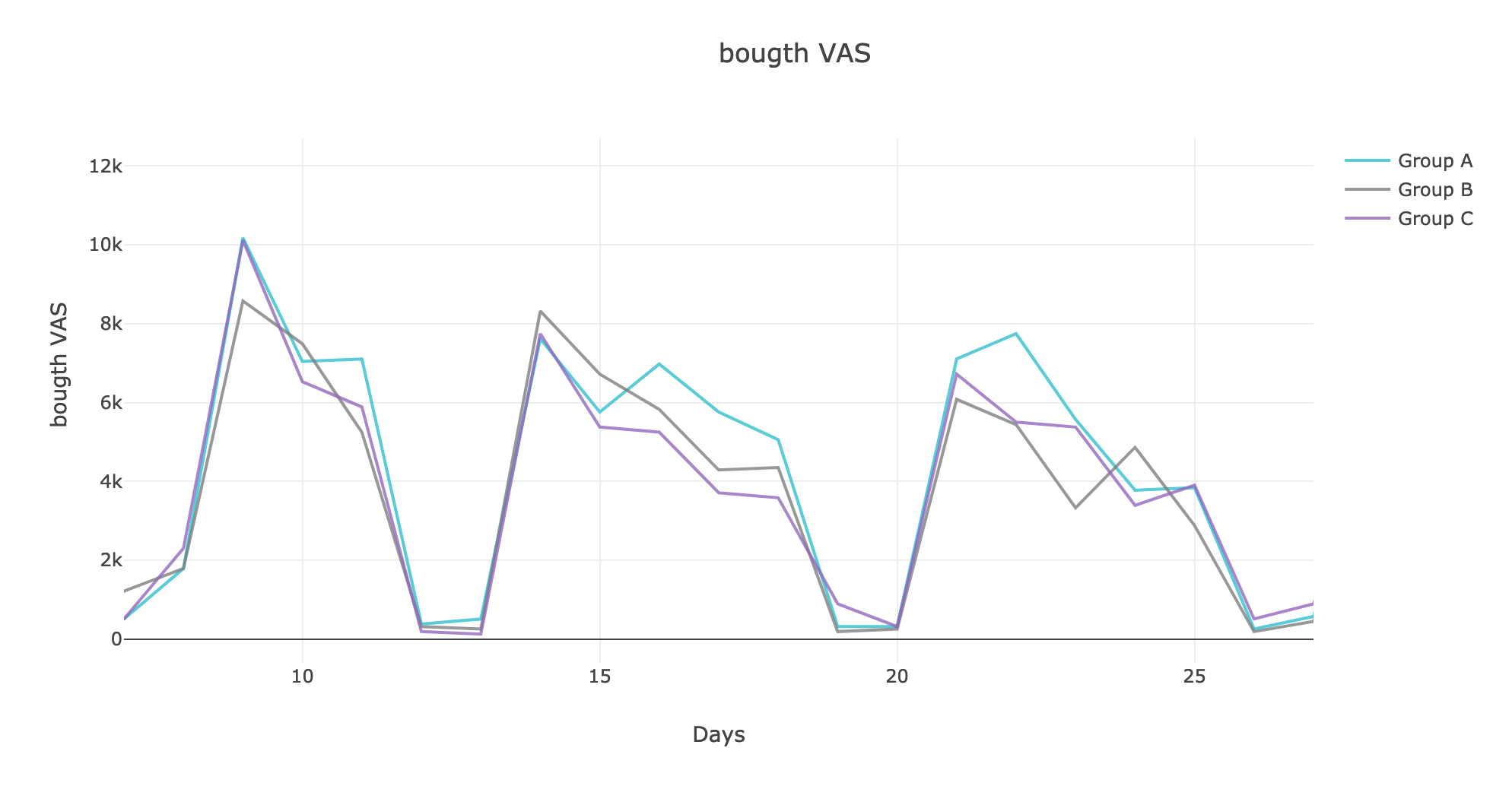
An experienced look will notice a weak predominance of group A in one of the weeks.
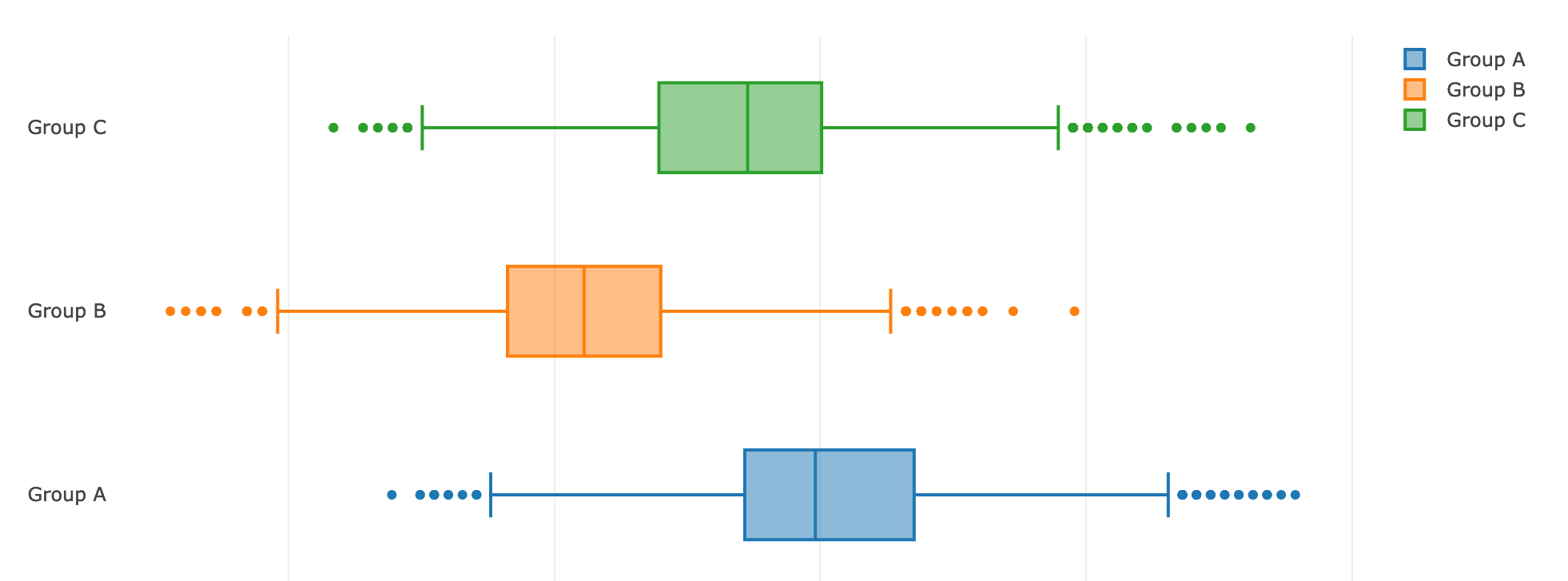
Let's look at the differences in the target actions, presenting the data in the form of box-plot'ov:

We see that the effect is indeed present, which means we need to evaluate how likely it is that the results really differ.
Initially, we will use the test to verify the equality of variances:
Test results are not stat. significant, therefore the variances in the subgroups are homogeneous. This time we used the Leven criterion, which is less sensitive to the deviation of the metric in the samples from the normal distribution than the Barlett criterion. By the way, Leven’s criterion was born in 1960 and will soon celebrate its 60th anniversary.
We will use the tests for normality, we will bring the distribution of our criterion in the sample to normal form using one of the methods described in our previous article and we will break down to a direct analysis of the statistical significance of the results.
A simple method for assessing the likelihood of a false positive experiment coloring. Its essence can be described by a simple formula:
The main disadvantage of this approach is that when the power of the criterion decreases, which increases the likelihood of accepting a false hypothesis.
This approach can be implemented using the simple “out of the box” method using Twitter Bootstrap:
Having received statistical estimates, we can draw conclusions about the presence or absence of differences between groups.
The Holm method can be called the development of the idea embodied in the Bonferroni correction method for multiple hypothesis testing. Its principle is quite simple: iterative testing of hypotheses until the threshold is reached .
By the way, after bootstraping, the histograms and graphs took a more readable form:

Another method that can be used to evaluate the results of a statistical test is the Kruskal-Wallis method. It can be found in the standard library.
The implementation of the verification with this method seemed elegant enough, I will tell you: you will need two more steps to carry out the verification, as well as an additional function from the statsmodels library module. I invite you to read an article about the method and implement this check yourself, you will like it :)
It should also be noted that similarly, you can use the Mann-Whitney criterion.
I want to ask a question to an inquisitive reader: how does the Mann-Whitney criterion differ from the Kruskal-Wallis criterion? It's simple, but I suggest you check your erudition and answer this question yourself :)
Why are we doing these cross-checks with different tests? The answer is obvious - you can try to conduct A / A and examine whether this test is suitable for our data, you can use the trick by breaking offline one group into subgroups and conducting a study of the sensitivity and accuracy of the test for them, or you can try to validate the tests with each other.
It should be noted that in pursuit of the search for stat. Significance in changing the target metric, analysts often miss an important fact - sometimes the studied change affects not only or not at all the metric that was planned to be increased / decreased, but to another: for example, our total money may grow, but the conversion may drop there are users who began to pay for a more expensive service or product, but we lost some of the users who brought us money. It should be understood that winning in the short term, in the long term, we can get a drawdown in revenue - perhaps the number of users who buy a more expensive service on the service is limited, and at some point in time we will run into the “ceiling” of the market. The second undesirable option in this case is that a more expensive product lasts longer than a cheaper FMCG and is purchased less often, which means we will run into market restrictions again.
It should be understood that if we operate with a large number of metrics, as is usually the case in Internet projects, then any of them will necessarily be painted over. In this case, the second step for making a decision can be both the construction of an additional model over the current test (which, as a rule, is more expensive in time), and the visual check with the eyes of the most important metrics - for example, the financial component.
Today is all that I wanted to tell you about.
All the best wishes!
As promised in the previous article , today we will continue our discussion of the methodologies used in A / B testing and consider methods for evaluating the results of multiple experiments. We will see that the methodologies are quite simple, and mathematical statistics are not so scary, and the main basis of all is analytical thinking and common sense. However, I would like to say a few words about what kind of business problems help to solve rigorous mathematical methods, whether you need them at this stage of your company’s development, and what pros and cons exist in Big analytics.
"Kati in prod for all 100" or how to save a couple of billion for his company
In any startup flying at insane speeds, decisions are made with the same speed, and the effect of a newly launched product feature is usually so financially tangible that additional evidence is not required.
However, at a certain point in time, the company reaches such a scale and audience reach that, firstly, the task of expanding and searching for new sources of financial growth in the market due to its limited resource intensity becomes more and more difficult, and, secondly, losses from wrong decisions become critical - because without a preliminary study, without taking into account the statistical error of its results, the killer feature, presented to a product with an audience of several million DAUs, can lead to a user outflow second, improve the bounce-rate and stupendous losses in product sales that are only multiplying in the long run. In such a situation, the quick-and-dirty approach of fast analytics ceases to be useful and should give way to the approach of thoughtful and slow, thorough data analysis.
In addition, in large services that set themselves the tasks of strategic long-term planning and competent distribution of financial investments between parts of the product, conducting short- and long-term experiments is one of the most important tasks. However, for the quality and reliability of the decision made, one often has to pay with speed.
It should be noted that despite the heading of this paragraph, the scope of A / B tests extends much further beyond the boundaries of product analytics: this is the analysis of the quality of forecast models to assess future return on investment, and the study of the effectiveness of financial investments in various parts of the product and its advertising channels promotions, distribution analytics, LTV forecasting, financial modeling, quality assessment of scoring''s implemented ML-models, ranking and much more.
Typology of experiments: what, when and why
There are two types of experiments: those conducted with independent samples that are as consistent as possible with respect to each other at the same moment in time and those conducted with dependent samples or with the same group, but at different times.
A typical A / B product experiment that studies the effect of a new feature on key metrics refers to experiments with independent samples. Investigation of the influence of a factor during which it is impossible to distinguish between groups that interacted with the source of impact and those that did not interact, and therefore, it is possible to evaluate the impact only on the basis of metrics before and after, refers to the study with dependent samples. An example of such a study is the analysis of the results of an advertising company on TV. Another option for conducting an experiment with dependent samples may be a study in the format of pairwise comparisons of elements between groups, in which each element of the control sample is assigned an element of the experimental sample.
There are also A / A experiments and inverse experiments. These topics are quite interesting, but we will not consider them in detail in the framework of this article.
In addition, experiments can be carried out both in A / B format and in the format of multiple comparisons, as stated in the title of the article. Since the typical methodologies for calculating the A / B experiment were considered earlier , in this article we will talk about the methodologies for calculating multiple experiments and recommendations on the boundaries of their use for solving business problems.
Multiple Experiments: pros and cons
As mentioned above, sometimes in practice, multiple comparisons are made
It should be noted that each new split group added to the study reduces its accuracy, reduces the representativeness of the sample, and also increases the likelihood of an error of the first kind: for simultaneously conducted experiments the level of statistical significance is at the accepted alpha level for one experiment of 5%.
Why do multiple experiments, if they reduce the accuracy of the results of our study?
The first reason may be the desire of the business as soon as possible and cheaper to get an answer, which decision should be made if there are several options, saving the time and cost of developing and implementing the experiment.
The second reason may be testing combinations - the simplest example: the user is offered a different mutual arrangement of the two elements on the landing page.
In addition, one of the tasks of conducting a multiple test, although controversial in terms of accuracy of assessment for a number of reasons, may be the desire to conduct A / A / B - conducting parallel studies of A / A and A / B in order to verify the reliability of the results and eliminate the probability of a false-positive result (recall the famous article by David Kodavi about A / A ).
Simple methods for evaluating multiple tests
Today we will consider a typical and widespread task of introducing a new feature in order to increase the company's revenue by increasing the number of targeted monetized actions. At the entrance, we have three groups of users who were offered 3 different delivery options with the offer to click on the call button for an ad.
To test multiple hypotheses, approaches from the theory of analysis of variance, otherwise called ANOVA, are used. Moreover, in most cases, calculation and verification of the group probability of an error of the first kind FWER occurs.
The essence of FWER is quite simple: we evaluate the likelihood of false-positive results, errors of the first kind. Based on the principle of constructing this criterion, several methods are used to evaluate the result of the statistical significance of the test. Consider the two simplest and most popular methods.
Let's look at how the metric in dynamics has changed, building graphs in the plotly interactive library:
An experienced look will notice a weak predominance of group A in one of the weeks.
Let's look at the differences in the target actions, presenting the data in the form of box-plot'ov:
We see that the effect is indeed present, which means we need to evaluate how likely it is that the results really differ.
Initially, we will use the test to verify the equality of variances:
stats.levene(df['action_count'][df['bucket'] == '0'], df['action_count'][df['bucket'] == '1'], df['action_count'][df['bucket'] == '2'])
Test results are not stat. significant, therefore the variances in the subgroups are homogeneous. This time we used the Leven criterion, which is less sensitive to the deviation of the metric in the samples from the normal distribution than the Barlett criterion. By the way, Leven’s criterion was born in 1960 and will soon celebrate its 60th anniversary.
We will use the tests for normality, we will bring the distribution of our criterion in the sample to normal form using one of the methods described in our previous article and we will break down to a direct analysis of the statistical significance of the results.
1. Bonferroni Amendment
A simple method for assessing the likelihood of a false positive experiment coloring. Its essence can be described by a simple formula:
The main disadvantage of this approach is that when the power of the criterion decreases, which increases the likelihood of accepting a false hypothesis.
This approach can be implemented using the simple “out of the box” method using Twitter Bootstrap:
bs_01_estims = bs.bootstrap_ab(df[(df['bucket']=='0')].action_count.values, df[(df['bucket']=='1')].action_count.values, bs_stats.mean, bs_compare.difference, num_iterations=5000, alpha=0.05/3, iteration_batch_size=100, scale_test_by=1, num_threads=4) bs_12_estims = bs.bootstrap_ab(df[(df['bucket']=='1')].action_count.values, df[(df['bucket']=='2')].action_count.values, bs_stats.mean, bs_compare.difference, num_iterations=5000, alpha=0.05/3, iteration_batch_size=100, scale_test_by=1, num_threads=4) bs_02_estims = bs.bootstrap_ab(df[(df['bucket']=='0')].action_count.values, df[(df['bucket']=='2')].action_count.values, bs_stats.mean, bs_compare.difference, num_iterations=5000, alpha=0.05/3, iteration_batch_size=100, scale_test_by=1, num_threads=4)
Having received statistical estimates, we can draw conclusions about the presence or absence of differences between groups.
2. Hill Method
The Holm method can be called the development of the idea embodied in the Bonferroni correction method for multiple hypothesis testing. Its principle is quite simple: iterative testing of hypotheses until the threshold is reached .
N_buckets = 3 for i in range(N_buckets): bs_data[i] = bs.bootstrap(df[(df['bucket']=='i')].action_count.values, stat_func=bs_stats.mean, num_iterations=10000, iteration_batch_size=300, return_distribution=True) print(stats.kstest(bs_data[i])) print(stats.shapiro(bs_data[i])) st_01, pval_01 = stats.ttest_ind(bs_data[0], bs_data[1]) st_12, pval_12 = stats.ttest_ind(bs_data[1], bs_data[2]) st_02, pval_02 = stats.ttest_ind(bs_data[0], bs_data[2])
By the way, after bootstraping, the histograms and graphs took a more readable form:
3. The Kruskal-Wallis Method
Another method that can be used to evaluate the results of a statistical test is the Kruskal-Wallis method. It can be found in the standard library.
scipy.stats
stats.kruskal()
The implementation of the verification with this method seemed elegant enough, I will tell you: you will need two more steps to carry out the verification, as well as an additional function from the statsmodels library module. I invite you to read an article about the method and implement this check yourself, you will like it :)
It should also be noted that similarly, you can use the Mann-Whitney criterion.
I want to ask a question to an inquisitive reader: how does the Mann-Whitney criterion differ from the Kruskal-Wallis criterion? It's simple, but I suggest you check your erudition and answer this question yourself :)
Why are we doing these cross-checks with different tests? The answer is obvious - you can try to conduct A / A and examine whether this test is suitable for our data, you can use the trick by breaking offline one group into subgroups and conducting a study of the sensitivity and accuracy of the test for them, or you can try to validate the tests with each other.
As an afterword and parting words
It should be noted that in pursuit of the search for stat. Significance in changing the target metric, analysts often miss an important fact - sometimes the studied change affects not only or not at all the metric that was planned to be increased / decreased, but to another: for example, our total money may grow, but the conversion may drop there are users who began to pay for a more expensive service or product, but we lost some of the users who brought us money. It should be understood that winning in the short term, in the long term, we can get a drawdown in revenue - perhaps the number of users who buy a more expensive service on the service is limited, and at some point in time we will run into the “ceiling” of the market. The second undesirable option in this case is that a more expensive product lasts longer than a cheaper FMCG and is purchased less often, which means we will run into market restrictions again.
It should be understood that if we operate with a large number of metrics, as is usually the case in Internet projects, then any of them will necessarily be painted over. In this case, the second step for making a decision can be both the construction of an additional model over the current test (which, as a rule, is more expensive in time), and the visual check with the eyes of the most important metrics - for example, the financial component.
Today is all that I wanted to tell you about.
All the best wishes!
All Articles