しかし、タスクを解決できないほど退屈なものにしない多くの詳細がまだ残っています。 特に、初心者の方で、ガイダンス、ステップバイステップ、目の前で実行され、最初から最後まで完了するプロジェクトが必要な場合は、時間がかかりすぎます。 このような場合、通常の「この明らかな部分をスキップする」という言い訳はありません。
この記事では、Dog Breed Identifierを作成するタスクを検討します。ニューラルネットワークを作成してトレーニングし、AndroidのJavaに移植してGoogle Playで公開します。
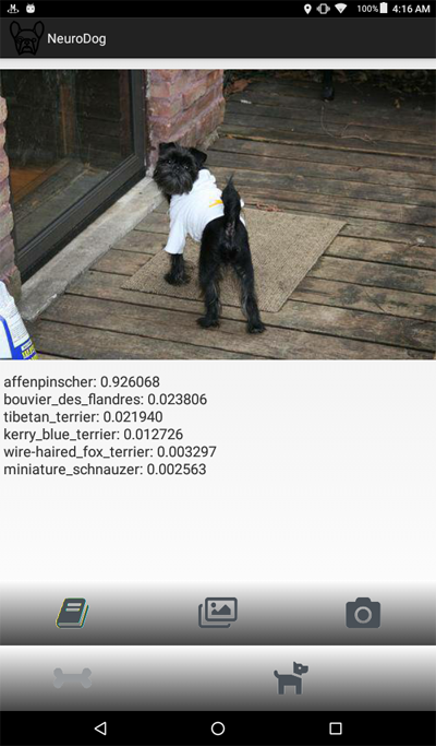
完成した結果をご覧になりたい場合は、Google PlayのNeuroDogアプリをご覧ください。
私のロボット(進行中)を含むWebサイト: robotics.snowcron.com 。
ガイドを含むプログラム自体のWebサイト: NeuroDog User Guide 。
そして、ここにプログラムのスクリーンショットがあります:
問題の声明
ニューラルネットワークを操作するためのGoogleライブラリであるKerasを使用します。 これは高レベルのライブラリです。つまり、私が知っている選択肢に比べて使いやすいです。 どちらかといえば-ネットワーク内のKerasには、高品質の教科書がたくさんあります。
CNN-Convolutional Neural Networksを使用します。 CNN(およびそれらに基づくより高度な構成)は、画像認識の事実上の標準です。 同時に、そのようなネットワークを訓練することは必ずしも容易ではありません。ネットワーク構造と訓練パラメーター(これらすべての学習率、運動量、L1およびL2など)を選択する必要があります。 このタスクにはかなりのコンピューティングリソースが必要なので、すべてのパラメーターを通過するだけで解決するには失敗します。
これは、ほとんどの場合、いわゆる「バニラ」アプローチの代わりに、いわゆる「転送知識」を使用する理由の1つです。 Transfer Knowlegeは、私たちの前の誰か(たとえば、Google)によって訓練されたニューラルネットワークを使用します。通常は、同様の、しかしまだ異なるタスクのために。 最初のレイヤーを取得し、最後のレイヤーを独自の分類子に置き換えます。そして、それが機能し、うまく機能します。
最初、そのような結果は驚くかもしれません:猫と椅子を区別するために訓練されたGoogleネットワークを利用して、犬の品種を認識しているのはどうしてでしょうか? これがどのように起こるかを理解するには、パターン認識に使用されるものを含む、ディープニューラルネットワークの基本原則を理解する必要があります。
入力として、ネットワークに画像(つまり、数字の配列)を「供給」しました。 最初のレイヤーは、水平線、円弧などの単純なパターンについて画像を分析します。 次の層は、これらのパターンを入力として受け取り、「毛皮」、「アイアングル」などの2次パターンを生成します。最終的に、犬を再構築できるパズルを取得します。
上記のすべては、(Googleなどから)私たちが取得した事前にトレーニングされたレイヤーの助けを借りて行われました。 次に、レイヤーを追加し、これらのパターンから品種情報を抽出することを教えます。 それは論理的に聞こえます。
要約すると、この記事では、「バニラ」CNNと、さまざまなタイプのネットワークの「転送学習」バリアントの両方を作成します。 「バニラ」については、作成しますが、「事前トレーニング済み」ネットワークのトレーニングと構成がはるかに簡単なので、パラメーターを選択して構成する予定はありません。
犬の品種を認識するようにニューラルネットワークを教える予定なので、さまざまな品種のサンプルを「表示」する必要があります。 幸いなことに、同様のタスクのためにここで作成された一連の写真があります( オリジナルはこちらです )。
次に、受信したネットワークのベストをAndroidに移植する予定です。 KerasovネットワークをAndroidに移植することは比較的単純で、十分に形式化されており、必要なすべての手順を実行するため、この部分を再現することは難しくありません。
その後、これらすべてをGoogle Playで公開します。 当然、グーグルは抵抗するので、追加のトリックが使用されます。 たとえば、アプリケーションのサイズ(巨大なニューラルネットワークによる)は、Google Playで受け入れられるAndroid APKの許容サイズよりも大きくなります。バンドルを使用する必要があります。 さらに、Googleは検索結果にアプリケーションを表示しません。これは、アプリケーションに検索タグを登録するか、1〜2週間待つだけで修正できます。
その結果、完全に機能する「商用」(引用符で囲まれ、無料で配置される)アプリケーションが、Androidおよびニューラルネットワークを使用して取得されます。
開発環境
Kerasのプログラムは、使用しているOS(Ubuntu推奨)、ビデオカードの有無などに応じて、さまざまな方法でプログラミングできます。 これが最も簡単な方法ではないことを除いて、ローカルコンピューターで開発するのは悪くありません(したがって、構成します)。
最初に、多数のツールとライブラリのインストールと構成に時間がかかります。次に、新しいバージョンがリリースされると、再び時間を費やす必要があります。 第二に、ニューラルネットワークはトレーニングに大きな計算能力を必要とします。 GPUを使用すると、このプロセスを(10倍以上)高速化できます。この記事の執筆時点では、この作業に最適なトップGPUの価格は2,000〜7,000ドルです。 はい、それらも構成する必要があります。
だから私たちは他の方法で行きます。 事実、Googleは私たちのような貧弱なハリネズミがクラスターのGPUを使用できることを許可しています-無料で、ニューラルネットワークに関連する計算のために、完全に構成された環境も提供します。 このサービスを使用すると、python、Keras、および既に構成されている膨大な数のライブラリを含むJupiter Notebookにアクセスできます。 Googleアカウントを取得するだけです(Gmailアカウントを取得すると、他のすべてにアクセスできます)。
現時点では、 ここでColabを雇うことができますが、Googleを知っていれば、これはいつでも変更できます。 Google Colabを検索するだけです。
Colabの使用に関する明らかな問題は、それがWEBサービスであることです。 どのようにデータにアクセスしますか? トレーニング後にニューラルネットワークを保存します。たとえば、タスク固有のデータをダウンロードしますか?
いくつかの方法(この記事の執筆時点では3つ)があり、最も便利だと思われる方法を使用しています。Googleドライブを使用しています。
Googleドライブは、通常のハードドライブとほとんど同じように機能するクラウドベースのデータストレージであり、Google Colabにマッピングできます(以下のコードを参照)。 その後、ローカルディスク上のファイルを操作するのと同じように操作できます。 つまり、たとえば、ニューラルネットワークをトレーニングするために犬の写真にアクセスするには、それらをGoogleドライブにアップロードする必要があります。それだけです。
ニューラルネットワークの作成とトレーニング
以下に、Pythonのコードをブロックごとに示します(Jupiter Notebookより)。 ブロックは独立して実行できるため、このコードをJupiter Notebookにコピーしてブロック単位で実行することもできます(もちろん、初期のブロックで定義された変数は後のブロックで必要になる場合がありますが、これは明らかな依存関係です)。
初期化
まず、Googleドライブをマウントしましょう。 わずか2行です。 このコードは、Colabセッションで1回だけ実行する必要があります(たとえば、6時間の作業で1回)。 セッションがまだ「生きている」間にもう一度呼び出すと、ディスクがすでにマウントされているためスキップされます。
from google.colab import drive drive.mount('/content/drive/')
最初の開始時には、意図を確認するように求められますが、複雑なことは何もありません。 これは次のようなものです。
>>> Go to this URL in a browser: ... >>> Enter your authorization code: >>> ·········· >>> Mounted at /content/drive/
完全に標準のincludeセクション。 含まれているファイルの一部が不要である可能性があります。 また、さまざまなニューラルネットワークをテストするため、特定のタイプのニューラルネットワークに含まれるモジュールの一部をコメント化/コメント解除する必要があります(たとえば、InceptionV3 NNを使用して、InceptionV3のインクルードをコメント解除し、たとえばResNet50をコメントアウトします)。 かどうか:これからのすべての変更は、使用されるメモリのサイズであり、それはあまり強くありません。
import datetime as dt import pandas as pd import seaborn as sns import matplotlib.pyplot as plt from tqdm import tqdm import cv2 import numpy as np import os import sys import random import warnings from sklearn.model_selection import train_test_split import keras from keras import backend as K from keras import regularizers from keras.models import Sequential from keras.models import Model from keras.layers import Dense, Dropout, Activation from keras.layers import Flatten, Conv2D from keras.layers import MaxPooling2D from keras.layers import BatchNormalization, Input from keras.layers import Dropout, GlobalAveragePooling2D from keras.callbacks import Callback, EarlyStopping from keras.callbacks import ReduceLROnPlateau from keras.callbacks import ModelCheckpoint import shutil from keras.applications.vgg16 import preprocess_input from keras.preprocessing import image from keras.preprocessing.image import ImageDataGenerator from keras.models import load_model from keras.applications.resnet50 import ResNet50 from keras.applications.resnet50 import preprocess_input from keras.applications.resnet50 import decode_predictions from keras.applications import inception_v3 from keras.applications.inception_v3 import InceptionV3 from keras.applications.inception_v3 import preprocess_input as inception_v3_preprocessor from keras.applications.mobilenetv2 import MobileNetV2 from keras.applications.nasnet import NASNetMobile
Googleドライブでは、ファイル用のフォルダーを作成します。 2行目には、その内容が表示されます。
working_path = "/content/drive/My Drive/DeepDogBreed/data/" !ls "/content/drive/My Drive/DeepDogBreed/data" >>> all_images labels.csv models test train valid
ご覧のとおり、犬の写真(Googleドライブのスタンフォードデータセット(上記参照)からコピー)は、最初にall_imagesフォルダーに保存されます。 後で、それらをtrain、validおよびtestディレクトリにコピーします。 トレーニング済みのモデルをモデルフォルダーに保存します。 labels.csvファイルに関しては、これは写真付きのデータセットの一部であり、写真と犬種の名前の対応表が含まれています。
Googleから一時的に使用するために得られたものを正確に把握するために実行できるテストは多数あります。 例:
# Is GPU Working? import tensorflow as tf tf.test.gpu_device_name() >>> '/device:GPU:0'
ご覧のとおり、GPUは実際に接続されています。接続されていない場合は、Jupiter Notebook設定でこのオプションを見つけて有効にする必要があります。
次に、画像のサイズなど、いくつかの定数を宣言する必要があります。 256x256ピクセルのサイズの写真を使用します。これは、細部を失わないように十分に大きい画像であり、すべてがメモリに収まるほど小さい画像です。 ただし、使用するニューラルネットワークの種類には、224x224ピクセルの画像が必要です。 そのような場合、256をコメントし、224のコメントを外します。
同じ方法(コメント1-コメント解除)を、保存するモデルの名前に適用します。これは、有用なファイルを上書きしたくないからです。
warnings.filterwarnings("ignore") os.environ['TF_CPP_MIN_LOG_LEVEL'] = '2' np.random.seed(7) start = dt.datetime.now() BATCH_SIZE = 16 EPOCHS = 15 TESTING_SPLIT=0.3 # 70/30 % NUM_CLASSES = 120 IMAGE_SIZE = 256 #strModelFileName = "models/ResNet50.h5" # strModelFileName = "models/InceptionV3.h5" strModelFileName = "models/InceptionV3_Sgd.h5" #IMAGE_SIZE = 224 #strModelFileName = "models/MobileNetV2.h5" #IMAGE_SIZE = 224 #strModelFileName = "models/NASNetMobileSgd.h5"
データの読み込み
まず、labels.csvファイルをアップロードして、トレーニングと検証の部分に分けましょう。 さらに多くのトレーニングデータを取得するためにチートを行うため、まだテスト部分はありません。
labels = pd.read_csv(working_path + 'labels.csv') print(labels.head()) train_ids, valid_ids = train_test_split(labels, test_size = TESTING_SPLIT) print(len(train_ids), 'train ids', len(valid_ids), 'validation ids') print('Total', len(labels), 'testing images') >>> id breed >>> 0 000bec180eb18c7604dcecc8fe0dba07 boston_bull >>> 1 001513dfcb2ffafc82cccf4d8bbaba97 dingo >>> 2 001cdf01b096e06d78e9e5112d419397 pekinese >>> 3 00214f311d5d2247d5dfe4fe24b2303d bluetick >>> 4 0021f9ceb3235effd7fcde7f7538ed62 golden_retriever >>> 7155 train ids 3067 validation ids >>> Total 10222 testing images
次に、ファイル名に従って、画像ファイルをトレーニング/検証/テストフォルダーにコピーします。 次の関数は、指定したフォルダーに名前を転送するファイルをコピーします。
def copyFileSet(strDirFrom, strDirTo, arrFileNames): arrBreeds = np.asarray(arrFileNames['breed']) arrFileNames = np.asarray(arrFileNames['id']) if not os.path.exists(strDirTo): os.makedirs(strDirTo) for i in tqdm(range(len(arrFileNames))): strFileNameFrom = strDirFrom + arrFileNames[i] + ".jpg" strFileNameTo = strDirTo + arrBreeds[i] + "/" + arrFileNames[i] + ".jpg" if not os.path.exists(strDirTo + arrBreeds[i] + "/"): os.makedirs(strDirTo + arrBreeds[i] + "/") # As a new breed dir is created, copy 1st file # to "test" under name of that breed if not os.path.exists(working_path + "test/"): os.makedirs(working_path + "test/") strFileNameTo = working_path + "test/" + arrBreeds[i] + ".jpg" shutil.copy(strFileNameFrom, strFileNameTo) shutil.copy(strFileNameFrom, strFileNameTo)
ご覧のとおり、 テストとして犬種ごとに1つのファイルのみをコピーします。 また、コピーするとき、サブフォルダを作成します(各品種に1つ)。 したがって、写真は品種ごとにサブフォルダーにコピーされます。
これは、Kerasが同様の構造のディレクトリを操作し、必要に応じて画像ファイルをロードできるため、一度にすべてではなくメモリを節約できるためです。 15,000枚すべての画像を一度にアップロードすることはお勧めできません。
この関数は画像をコピーするので、一度だけ呼び出す必要があります-もはや必要ありません。 したがって、将来の使用のために、コメントする必要があります。
# Move the data in subfolders so we can # use the Keras ImageDataGenerator. # This way we can also later use Keras # Data augmentation features. # --- Uncomment once, to copy files --- #copyFileSet(working_path + "all_images/", # working_path + "train/", train_ids) #copyFileSet(working_path + "all_images/", # working_path + "valid/", valid_ids)
犬の品種のリストを取得します。
breeds = np.unique(labels['breed']) map_characters = {} #{0:'none'} for i in range(len(breeds)): map_characters[i] = breeds[i] print("<item>" + breeds[i] + "</item>") >>> <item>affenpinscher</item> >>> <item>afghan_hound</item> >>> <item>african_hunting_dog</item> >>> <item>airedale</item> >>> <item>american_staffordshire_terrier</item> >>> <item>appenzeller</item>
画像処理
ImageDataGeneratorsと呼ばれるKerasライブラリ機能を使用します。 ImageDataGeneratorは、画像の処理、拡大縮小、回転などを行うことができます。 また、画像をさらに処理できる処理機能を受け入れることもできます。
def preprocess(img): img = cv2.resize(img, (IMAGE_SIZE, IMAGE_SIZE), interpolation = cv2.INTER_AREA) # or use ImageDataGenerator( rescale=1./255... img_1 = image.img_to_array(img) img_1 = cv2.resize(img_1, (IMAGE_SIZE, IMAGE_SIZE), interpolation = cv2.INTER_AREA) img_1 = np.expand_dims(img_1, axis=0) / 255. #img = cv2.blur(img,(5,5)) return img_1[0]
次のコードに注意してください。
# or use ImageDataGenerator( rescale=1./255...
ImageDataGenerator自体で正規化できます(元の0-255ではなく、0-1の範囲のサブデータ)。 なぜプリプロセッサが必要なのですか? 例として、不鮮明な呼び出しを検討します(コメント化されていますが、使用しません)。これは、任意のカスタム画像操作と同じです。 HDRとは対照的なもの。
トレーニング用と検証用の2つの異なるImageDataGeneratorを使用します。 違いは、トレーニングにはデータの「多様性」を高めるためにターンとスケーリングが必要ですが、検証には少なくともこのタスクでは必要ないということです。
train_datagen = ImageDataGenerator( preprocessing_function=preprocess, #rescale=1./255, # done in preprocess() # randomly rotate images (degrees, 0 to 30) rotation_range=30, # randomly shift images horizontally # (fraction of total width) width_shift_range=0.3, height_shift_range=0.3, # randomly flip images horizontal_flip=True, ,vertical_flip=False, zoom_range=0.3) val_datagen = ImageDataGenerator( preprocessing_function=preprocess) train_gen = train_datagen.flow_from_directory( working_path + "train/", batch_size=BATCH_SIZE, target_size=(IMAGE_SIZE, IMAGE_SIZE), shuffle=True, class_mode="categorical") val_gen = val_datagen.flow_from_directory( working_path + "valid/", batch_size=BATCH_SIZE, target_size=(IMAGE_SIZE, IMAGE_SIZE), shuffle=True, class_mode="categorical")
ニューラルネットワークの作成
既に述べたように、いくつかのタイプのニューラルネットワークを作成します。 別の関数を呼び出して作成し、他のファイルをインクルードし、時には異なる画像サイズを決定するたびに。 したがって、異なるタイプのニューラルネットワークを切り替えるには、適切なコードをコメント化/コメント解除する必要があります。
まず、「バニラ」CNNを作成します。 デバッグに時間を浪費しないことに決めたため、うまくいきませんが、少なくとも要望があれば開発できる基礎を提供します(通常、事前訓練されたネットワークが最良の結果をもたらすため、これは悪い考えです)。
def createModelVanilla(): model = Sequential() # Note the (7, 7) here. This is one of technics # used to reduce memory use by the NN: we scan # the image in a larger steps. # Also note regularizers.l2: this technic is # used to prevent overfitting. The "0.001" here # is an empirical value and can be optimized. model.add(Conv2D(16, (7, 7), padding='same', use_bias=False, input_shape=(IMAGE_SIZE, IMAGE_SIZE, 3), kernel_regularizer=regularizers.l2(0.001))) # Note the use of a standard CNN building blocks: # Conv2D - BatchNormalization - Activation # MaxPooling2D - Dropout # The last two are used to avoid overfitting, also, # MaxPooling2D reduces memory use. model.add(BatchNormalization(axis=3, scale=False)) model.add(Activation("relu")) model.add(MaxPooling2D(pool_size=(2, 2), strides=(2, 2), padding='same')) model.add(Dropout(0.5)) model.add(Conv2D(16, (3, 3), padding='same', use_bias=False, kernel_regularizer=regularizers.l2(0.01))) model.add(BatchNormalization(axis=3, scale=False)) model.add(Activation("relu")) model.add(MaxPooling2D(pool_size=(2, 2), strides=(1, 1), padding='same')) model.add(Dropout(0.5)) model.add(Conv2D(32, (3, 3), padding='same', use_bias=False, kernel_regularizer=regularizers.l2(0.01))) model.add(BatchNormalization(axis=3, scale=False)) model.add(Activation("relu")) model.add(Dropout(0.5)) model.add(Conv2D(32, (3, 3), padding='same', use_bias=False, kernel_regularizer=regularizers.l2(0.01))) model.add(BatchNormalization(axis=3, scale=False)) model.add(Activation("relu")) model.add(MaxPooling2D(pool_size=(2, 2), strides=(1, 1), padding='same')) model.add(Dropout(0.5)) model.add(Conv2D(64, (3, 3), padding='same', use_bias=False, kernel_regularizer=regularizers.l2(0.01))) model.add(BatchNormalization(axis=3, scale=False)) model.add(Activation("relu")) model.add(Dropout(0.5)) model.add(Conv2D(64, (3, 3), padding='same', use_bias=False, kernel_regularizer=regularizers.l2(0.01))) model.add(BatchNormalization(axis=3, scale=False)) model.add(Activation("relu")) model.add(MaxPooling2D(pool_size=(2, 2), strides=(1, 1), padding='same')) model.add(Dropout(0.5)) model.add(Conv2D(128, (3, 3), padding='same', use_bias=False, kernel_regularizer=regularizers.l2(0.01))) model.add(BatchNormalization(axis=3, scale=False)) model.add(Activation("relu")) model.add(Dropout(0.5)) model.add(Conv2D(128, (3, 3), padding='same', use_bias=False, kernel_regularizer=regularizers.l2(0.01))) model.add(BatchNormalization(axis=3, scale=False)) model.add(Activation("relu")) model.add(MaxPooling2D(pool_size=(2, 2), strides=(1, 1), padding='same')) model.add(Dropout(0.5)) model.add(Conv2D(256, (3, 3), padding='same', use_bias=False, kernel_regularizer=regularizers.l2(0.01))) model.add(BatchNormalization(axis=3, scale=False)) model.add(Activation("relu")) model.add(Dropout(0.5)) model.add(Conv2D(256, (3, 3), padding='same', use_bias=False, kernel_regularizer=regularizers.l2(0.01))) model.add(BatchNormalization(axis=3, scale=False)) model.add(Activation("relu")) model.add(MaxPooling2D(pool_size=(2, 2), strides=(1, 1), padding='same')) model.add(Dropout(0.5)) # This is the end on "convolutional" part of CNN. # Now we need to transform multidementional # data into one-dim. array for a fully-connected # classifier: model.add(Flatten()) # And two layers of classifier itself (plus an # Activation layer in between): model.add(Dense(NUM_CLASSES, activation='softmax', kernel_regularizer=regularizers.l2(0.01))) model.add(Activation("relu")) model.add(Dense(NUM_CLASSES, activation='softmax', kernel_regularizer=regularizers.l2(0.01))) # We need to compile the resulting network. # Note that there are few parameters we can # try here: the best performing one is uncommented, # the rest is commented out for your reference. #model.compile(optimizer='rmsprop', # loss='categorical_crossentropy', # metrics=['accuracy']) #model.compile( # optimizer=keras.optimizers.RMSprop(lr=0.0005), # loss='categorical_crossentropy', # metrics=['accuracy']) model.compile(optimizer='adam', loss='categorical_crossentropy', metrics=['accuracy']) #model.compile(optimizer='adadelta', # loss='categorical_crossentropy', # metrics=['accuracy']) #opt = keras.optimizers.Adadelta(lr=1.0, # rho=0.95, epsilon=0.01, decay=0.01) #model.compile(optimizer=opt, # loss='categorical_crossentropy', # metrics=['accuracy']) #opt = keras.optimizers.RMSprop(lr=0.0005, # rho=0.9, epsilon=None, decay=0.0001) #model.compile(optimizer=opt, # loss='categorical_crossentropy', # metrics=['accuracy']) # model.summary() return(model)
転送学習を使用してネットワークを作成すると、手順が変わります。
def createModelMobileNetV2(): # First, create the NN and load pre-trained # weights for it ('imagenet') # Note that we are not loading last layers of # the network (include_top=False), as we are # going to add layers of our own: base_model = MobileNetV2(weights='imagenet', include_top=False, pooling='avg', input_shape=(IMAGE_SIZE, IMAGE_SIZE, 3)) # Then attach our layers at the end. These are # to build "classifier" that makes sense of # the patterns previous layers provide: x = base_model.output x = Dense(512)(x) x = Activation('relu')(x) x = Dropout(0.5)(x) predictions = Dense(NUM_CLASSES, activation='softmax')(x) # Create a model model = Model(inputs=base_model.input, outputs=predictions) # We need to make sure that pre-trained # layers are not changed when we train # our classifier: # Either this: #model.layers[0].trainable = False # or that: for layer in base_model.layers: layer.trainable = False # As always, there are different possible # settings, I tried few and chose the best: # model.compile(optimizer='adam', # loss='categorical_crossentropy', # metrics=['accuracy']) model.compile(optimizer='sgd', loss='categorical_crossentropy', metrics=['accuracy']) #model.summary() return(model)
他のタイプのネットワークの作成も同じパターンに従います。
def createModelResNet50(): base_model = ResNet50(weights='imagenet', include_top=False, pooling='avg', input_shape=(IMAGE_SIZE, IMAGE_SIZE, 3)) x = base_model.output x = Dense(512)(x) x = Activation('relu')(x) x = Dropout(0.5)(x) predictions = Dense(NUM_CLASSES, activation='softmax')(x) model = Model(inputs=base_model.input, outputs=predictions) #model.layers[0].trainable = False # model.compile(loss='categorical_crossentropy', # optimizer='adam', metrics=['accuracy']) model.compile(optimizer='sgd', loss='categorical_crossentropy', metrics=['accuracy']) #model.summary() return(model)
警告:勝者! このNNは最高の結果を示しました。
def createModelInceptionV3(): # model.layers[0].trainable = False # model.compile(optimizer='sgd', # loss='categorical_crossentropy', # metrics=['accuracy']) base_model = InceptionV3(weights = 'imagenet', include_top = False, input_shape=(IMAGE_SIZE, IMAGE_SIZE, 3)) x = base_model.output x = GlobalAveragePooling2D()(x) x = Dense(512, activation='relu')(x) predictions = Dense(NUM_CLASSES, activation='softmax')(x) model = Model(inputs = base_model.input, outputs = predictions) for layer in base_model.layers: layer.trainable = False # model.compile(optimizer='adam', # loss='categorical_crossentropy', # metrics=['accuracy']) model.compile(optimizer='sgd', loss='categorical_crossentropy', metrics=['accuracy']) #model.summary() return(model)
別のもの:
def createModelNASNetMobile(): # model.layers[0].trainable = False # model.compile(optimizer='sgd', # loss='categorical_crossentropy', # metrics=['accuracy']) base_model = NASNetMobile(weights = 'imagenet', include_top = False, input_shape=(IMAGE_SIZE, IMAGE_SIZE, 3)) x = base_model.output x = GlobalAveragePooling2D()(x) x = Dense(512, activation='relu')(x) predictions = Dense(NUM_CLASSES, activation='softmax')(x) model = Model(inputs = base_model.input, outputs = predictions) for layer in base_model.layers: layer.trainable = False # model.compile(optimizer='adam', # loss='categorical_crossentropy', # metrics=['accuracy']) model.compile(optimizer='sgd', loss='categorical_crossentropy', metrics=['accuracy']) #model.summary() return(model)
さまざまな種類のニューラルネットワークをさまざまなタスクに使用できます。 そのため、予測精度の要件に加えて、サイズ(モバイルNNはInceptionの5倍)と速度が重要です(ビデオストリームのリアルタイム処理が必要な場合は、精度を犠牲にする必要があります)。
ニューラルネットワークトレーニング
まず、 実験中ですので、保存したが使用しなくなったニューラルネットワークを削除できるはずです。 次の関数は、NNが存在する場合は削除します。
# Make sure that previous "best network" is deleted. def deleteSavedNet(best_weights_filepath): if(os.path.isfile(best_weights_filepath)): os.remove(best_weights_filepath) print("deleteSavedNet():File removed") else: print("deleteSavedNet():No file to remove")
ニューラルネットワークを作成および削除する方法は、非常にシンプルで簡単です。 まず、削除します。 delete (のみ)を呼び出す場合、Jupiter Notebookには「実行選択」機能があり、使用するもののみを選択して実行することに注意してください。
次に、ファイルが存在しない場合はニューラルネットワークを作成し、ファイルが存在する場合はloadを呼び出します 。もちろん、「delete」を呼び出してNNが存在することを期待できないため、保存されたニューラルネットワークを使用するにはdeleteを呼び出さないでください 。
言い換えれば、状況と現在実験していることに応じて、新しいNNを作成するか、既存のNNを使用できます。 単純なシナリオ:ニューラルネットワークをトレーニングし、その後休暇を取りました。 それらが返され、Googleがセッションを釘付けにしたので、以前に保存したものをロードする必要があります。「delete」をコメントアウトし、「load」のコメントを外します。
deleteSavedNet(working_path + strModelFileName) #if not os.path.exists(working_path + "models"): # os.makedirs(working_path + "models") # #if not os.path.exists(working_path + # strModelFileName): # model = createModelResNet50() model = createModelInceptionV3() # model = createModelMobileNetV2() # model = createModelNASNetMobile() #else: # model = load_model(working_path + strModelFileName)
チェックポイントはプログラムの非常に重要な要素です。 トレーニングの各時代の終わりに呼び出される関数の配列を作成し、チェックポイントに渡すことができます。 たとえば、既に保存されている結果よりも良い結果を示す場合 、ニューラルネットワークを保存できます。
checkpoint = ModelCheckpoint(working_path + strModelFileName, monitor='val_acc', verbose=1, save_best_only=True, mode='auto', save_weights_only=False) callbacks_list = [ checkpoint ]
最後に、トレーニングセットでニューラルネットワークを学習します。
# Calculate sizes of training and validation sets STEP_SIZE_TRAIN=train_gen.n//train_gen.batch_size STEP_SIZE_VALID=val_gen.n//val_gen.batch_size # Set to False if we are experimenting with # some other part of code, use history that # was calculated before (and is still in # memory bDoTraining = True if bDoTraining == True: # model.fit_generator does the actual training # Note the use of generators and callbacks # that were defined earlier history = model.fit_generator(generator=train_gen, steps_per_epoch=STEP_SIZE_TRAIN, validation_data=val_gen, validation_steps=STEP_SIZE_VALID, epochs=EPOCHS, callbacks=callbacks_list) # --- After fitting, load the best model # This is important as otherwise we'll # have the LAST model loaded, not necessarily # the best one. model.load_weights(working_path + strModelFileName) # --- Presentation part # summarize history for accuracy plt.plot(history.history['acc']) plt.plot(history.history['val_acc']) plt.title('model accuracy') plt.ylabel('accuracy') plt.xlabel('epoch') plt.legend(['acc', 'val_acc'], loc='upper left') plt.show() # summarize history for loss plt.plot(history.history['loss']) plt.plot(history.history['val_loss']) plt.title('model loss') plt.ylabel('loss') plt.xlabel('epoch') plt.legend(['loss', 'val_loss'], loc='upper left') plt.show() # As grid optimization of NN would take too long, # I did just few tests with different parameters. # Below I keep results, commented out, in the same # code. As you can see, Inception shows the best # results: # Inception: # adam: val_acc 0.79393 # sgd: val_acc 0.80892 # Mobile: # adam: val_acc 0.65290 # sgd: Epoch 00015: val_acc improved from 0.67584 to 0.68469 # sgd-30 epochs: 0.68 # NASNetMobile, adam: val_acc did not improve from 0.78335 # NASNetMobile, sgd: 0.8
最高の構成の精度と損失のグラフは次のとおりです。
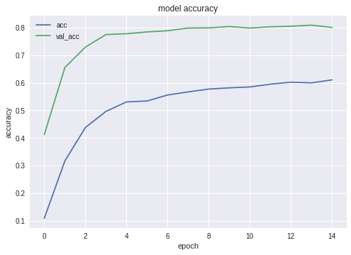

ご覧のとおり、ニューラルネットワークは学習中で、非常にうまく機能しています。
ニューラルネットワークのテスト
トレーニングが完了したら、結果をテストする必要があります。 このため、NNは、これまでに見たことのない写真(テストフォルダーにコピーしたもの)を犬種ごとに1枚提示します。
# --- Test j = 0 # Final cycle performs testing on the entire # testing set. for file_name in os.listdir( working_path + "test/"): img = image.load_img(working_path + "test/" + file_name); img_1 = image.img_to_array(img) img_1 = cv2.resize(img_1, (IMAGE_SIZE, IMAGE_SIZE), interpolation = cv2.INTER_AREA) img_1 = np.expand_dims(img_1, axis=0) / 255. y_pred = model.predict_on_batch(img_1) # get 5 best predictions y_pred_ids = y_pred[0].argsort()[-5:][::-1] print(file_name) for i in range(len(y_pred_ids)): print("\n\t" + map_characters[y_pred_ids[i]] + " (" + str(y_pred[0][y_pred_ids[i]]) + ")") print("--------------------\n") j = j + 1
ニューラルネットワークをJavaアプリケーションにエクスポートする
まず、ディスクからのニューラルネットワークの読み込みを整理する必要があります。 その理由は明らかです。エクスポートは別のコードブロックで行われるため、ニューラルネットワークが最適な状態になったときにエクスポートを個別に開始する可能性が高くなります。 つまり、エクスポートの直前に、プログラムの同じ実行で、ネットワークをトレーニングしません。 ここに示すコードを使用する場合、違いはなく、最適なネットワークが選択されています。 しかし、自分で何かを学んだ場合、すべてを保存する前に、保存する前にすべてを新しく訓練するのは時間の無駄です。
# Test: load and run model = load_model(working_path + strModelFileName)
同じ理由で-コードを飛び越えないために-エクスポートに必要なファイルをここに含めます。 あなたの美しさの感覚がそれを必要とするならば、誰もあなたをプログラムの始めにそれらを動かすことを気にしません:
from keras.models import Model from keras.models import load_model from keras.layers import * import os import sys import tensorflow as tf
ニューラルネットワークをロードした後の小さなテスト。すべてがロードされていることを確認するためだけです。
img = image.load_img(working_path + "test/affenpinscher.jpg") #basset.jpg") img_1 = image.img_to_array(img) img_1 = cv2.resize(img_1, (IMAGE_SIZE, IMAGE_SIZE), interpolation = cv2.INTER_AREA) img_1 = np.expand_dims(img_1, axis=0) / 255. y_pred = model.predict(img_1) Y_pred_classes = np.argmax(y_pred,axis = 1) # print(y_pred) fig, ax = plt.subplots() ax.imshow(img) ax.axis('off') ax.set_title(map_characters[Y_pred_classes[0]]) plt.show()

次に、ネットワークの入力層と出力層の名前を取得する必要があります(この関数または作成関数のいずれかで、層に明示的に「名前を付ける」必要がありますが、行いません)。
model.summary() >>> Layer (type) >>> ====================== >>> input_7 (InputLayer) >>> ______________________ >>> conv2d_283 (Conv2D) >>> ______________________ >>> ... >>> dense_14 (Dense) >>> ====================== >>> Total params: 22,913,432 >>> Trainable params: 1,110,648 >>> Non-trainable params: 21,802,784
ニューラルネットワークをJavaアプリケーションにインポートするときに、入力層と出力層の名前を使用します。
このデータを取得するためにネットワークをローミングする別のコード:
def print_graph_nodes(filename): g = tf.GraphDef() g.ParseFromString(open(filename, 'rb').read()) print() print(filename) print("=======================INPUT===================") print([n for n in g.node if n.name.find('input') != -1]) print("=======================OUTPUT==================") print([n for n in g.node if n.name.find('output') != -1]) print("===================KERAS_LEARNING==============") print([n for n in g.node if n.name.find('keras_learning_phase') != -1]) print("===============================================") print() #def get_script_path(): # return os.path.dirname(os.path.realpath(sys.argv[0]))
しかし、私は彼が好きではなく、彼を推薦しません。
次のコードは、Keras Neural NetworkをAndroidからキャプチャするpb形式にエクスポートします。
def keras_to_tensorflow(keras_model, output_dir, model_name,out_prefix="output_", log_tensorboard=True): if os.path.exists(output_dir) == False: os.mkdir(output_dir) out_nodes = [] for i in range(len(keras_model.outputs)): out_nodes.append(out_prefix + str(i + 1)) tf.identity(keras_model.output[i], out_prefix + str(i + 1)) sess = K.get_session() from tensorflow.python.framework import graph_util from tensorflow.python.framework graph_io init_graph = sess.graph.as_graph_def() main_graph = graph_util.convert_variables_to_constants( sess, init_graph, out_nodes) graph_io.write_graph(main_graph, output_dir, name=model_name, as_text=False) if log_tensorboard: from tensorflow.python.tools import import_pb_to_tensorboard import_pb_to_tensorboard.import_to_tensorboard( os.path.join(output_dir, model_name), output_dir)
:
model = load_model(working_path + strModelFileName) keras_to_tensorflow(model, output_dir=working_path + strModelFileName, model_name=working_path + "models/dogs.pb") print_graph_nodes(working_path + "models/dogs.pb")
.
Android
Android . , , , ( ) .
, Android Studio . « », — . activity.
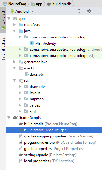
, «assets» (, ).
Gradle
. , tensorflow-android . , Tensorflow (, , Keras) Java:
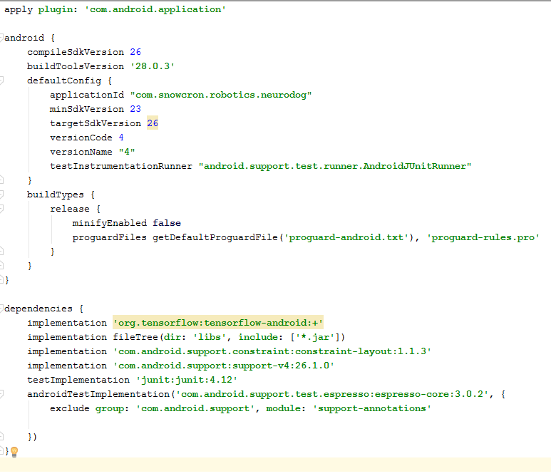
: versionCode versionName . , Google Play. gdadle (, 1 -> 2 -> 3...) , « ».
, «» — 100 Mb Neural Network , instance «» Facebook .
instance :
<activity android:name=".MainActivity" android:launchMode="singleTask">
android:launchMode=«singleTask» MainActivity, Android, () , , instance.
, , - «» :
<intent-filter> <!-- Send action required to display activity in share list --> <action android:name="android.intent.action.SEND" /> <!-- Make activity default to launch --> <category android:name="android.intent.category.DEFAULT" /> <!-- Mime type ie what can be shared with this activity only image and text --> <data android:mimeType="image/*" /> </intent-filter>
, , :
<uses-feature android:name="android.hardware.camera" android:required="true" /> <uses-permission android:name= "android.permission.WRITE_EXTERNAL_STORAGE" /> <uses-permission android:name="android.permission.READ_PHONE_STATE" tools:node="remove" />
Android, .
Layout .
layouts, , . Portrait layout .
: (view) , (, «»), «Help», File/Gallery , ( ) «Process» .
, enabling/disabling , .
MainActivity
activity (extends) Android Activity:
public class MainActivity extends Activity
, .
, Bitmap. , Bitmap ( ) (m_bitmap), , 256x256 (m_bitmapForNn). (256) :
static Bitmap m_bitmap = null; static Bitmap m_bitmapForNn = null; private int m_nImageSize = 256;
; (. ), , :
private String INPUT_NAME = "input_7_1"; private String OUTPUT_NAME = "output_1";
TensofFlow. , ( assets):
private TensorFlowInferenceInterface tf;
private String MODEL_PATH =
	"file:///android_asset/dogs.pb";
, , :
private String[] m_arrBreedsArray;
, Bitmap. , RGB , — , — , . , (, 120 , ):
private float[] m_arrPrediction = new float[120]; private float[] m_arrInput = null;
tensorflow inference library:
static { System.loadLibrary("tensorflow_inference"); }
, , , « », .
class PredictionTask extends AsyncTask<Void, Void, Void> { @Override protected void onPreExecute() { super.onPreExecute(); } // --- @Override protected Void doInBackground(Void... params) { try { # We get RGB values packed in integers # from the Bitmap, then break those # integers into individual triplets m_arrInput = new float[ m_nImageSize * m_nImageSize * 3]; int[] intValues = new int[ m_nImageSize * m_nImageSize]; m_bitmapForNn.getPixels(intValues, 0, m_nImageSize, 0, 0, m_nImageSize, m_nImageSize); for (int i = 0; i < intValues.length; i++) { int val = intValues[i]; m_arrInput[i * 3 + 0] = ((val >> 16) & 0xFF) / 255f; m_arrInput[i * 3 + 1] = ((val >> 8) & 0xFF) / 255f; m_arrInput[i * 3 + 2] = (val & 0xFF) / 255f; } // --- tf = new TensorFlowInferenceInterface( getAssets(), MODEL_PATH); //Pass input into the tensorflow tf.feed(INPUT_NAME, m_arrInput, 1, m_nImageSize, m_nImageSize, 3); //compute predictions tf.run(new String[]{OUTPUT_NAME}, false); //copy output into PREDICTIONS array tf.fetch(OUTPUT_NAME, m_arrPrediction); } catch (Exception e) { e.getMessage(); } return null; } // --- @Override protected void onPostExecute(Void result) { super.onPostExecute(result); // --- enableControls(true); // --- tf = null; m_arrInput = null; # strResult contains 5 lines of text # with most probable dog breeds and # their probabilities m_strResult = ""; # What we do below is sorting the array # by probabilities (using map) # and getting in reverse order) the # first five entries TreeMap<Float, Integer> map = new TreeMap<Float, Integer>( Collections.reverseOrder()); for(int i = 0; i < m_arrPrediction.length; i++) map.put(m_arrPrediction[i], i); int i = 0; for (TreeMap.Entry<Float, Integer> pair : map.entrySet()) { float key = pair.getKey(); int idx = pair.getValue(); String strBreed = m_arrBreedsArray[idx]; m_strResult += strBreed + ": " + String.format("%.6f", key) + "\n"; i++; if (i > 5) break; } m_txtViewBreed.setVisibility(View.VISIBLE); m_txtViewBreed.setText(m_strResult); } }
In onCreate() of the MainActivity, we need to add the onClickListener for the «Process» button:
m_btn_process.setOnClickListener(new View.OnClickListener() { @Override public void onClick(View v) { processImage(); } });
processImage() , :
private void processImage() { try { enableControls(false); // --- PredictionTask prediction_task = new PredictionTask(); prediction_task.execute(); } catch (Exception e) { e.printStackTrace(); } }
UI- , . , .
instances , (flow of control): «» Facebook, , . , «» onCreate , onCreate .
:
1. onCreate MainActivity, onSharedIntent:
protected void onCreate( Bundle savedInstanceState) { super.onCreate(savedInstanceState); .... onSharedIntent(); ....
onNewIntent:
@Override protected void onNewIntent(Intent intent) { super.onNewIntent(intent); setIntent(intent); onSharedIntent(); }
onSharedIntent:
private void onSharedIntent() { Intent receivedIntent = getIntent(); String receivedAction = receivedIntent.getAction(); String receivedType = receivedIntent.getType(); if (receivedAction.equals(Intent.ACTION_SEND)) { // If mime type is equal to image if (receivedType.startsWith("image/")) { m_txtViewBreed.setText(""); m_strResult = ""; Uri receivedUri = receivedIntent.getParcelableExtra( Intent.EXTRA_STREAM); if (receivedUri != null) { try { Bitmap bitmap = MediaStore.Images.Media.getBitmap( this.getContentResolver(), receivedUri); if(bitmap != null) { m_bitmap = bitmap; m_picView.setImageBitmap(m_bitmap); storeBitmap(); enableControls(true); } } catch (Exception e) { e.printStackTrace(); } } } } }
onCreate ( ) onNewIntent ( ).
頑張って , , «» , «» .