プログラミング言語Rを使用して、blablacar.ruサイトを解析し、ブリャンスク州クリンツィー市からの旅客トラフィックを分析します。

背景
さまざまな状況の意志により、彼はブリャンスク地方(クリンツィー)の小さな町にシフトダウンしました。 私は住んでいて、仕事をしていて、文化的な休日に興味があります。 「どこに行けばいいの?」地元の人に聞いた。 「チケットを買うには駅に行くのが最善です」と臨床医は親切にアドバイスします。
私はこのアイデアが気に入ったので、心配から離れて、この目的のためにブラブラカルを選択して、1日から2日旅行することにしました(理論的には、より経済的で、旅行時間を選択する方が簡単で、ドライバーと話すことができ、より多くのルートがあります)。
想像しやすくするために、どこで、いつ、どのように、どのくらいクリントシーを離れることができるかについて、私は小さな研究を実施しました。 この記事の結果、アルゴリズム、スクリプト、およびデータを共有します。
Rライブラリ
以下のRライブラリーが研究に使用されました。
- rvest、Rselenium-データ解析;
- dplyr、tidyr-データ操作。
- ggplot2、ggmap、grid、gridExtra-視覚化;
- 予測、動物園-時系列で動作します。
- aret、xgboost、mlr-機械学習。
データ検索
移動中に標準のRツール(rvestライブラリ)を使用してサイトからデータを収集することはできませんでした。 Blablacarは、ユーザーの要求に応じて動的ページを形成するJS上で実行されますが、rvest関数はそれらをサポートしません。
サーバーのどこに何があり、どのようにプルされているのか理解していない限り、Webテクノロジーに精通しているので、私は、よりシンプルなソリューションを選択しました。
Rseleniumサーバーをマシンにインストールし、それを介してGoogle Chromeを起動し、目的のページを作成して出力を保存しました。 さらに、ページは問題なく解析されましたR。
Blablacarが提供するデータはわずか2か月(713回)であるため、このスキームは正常に機能しました(3回目から松葉杖をきしむ音が鳴り、サーバーが起動しました)。 ただし、アルゴリズムがより多くのページを解析するのに適しているかどうかはわかりません。多くの時間とリソースが費やされ、多くのボトルネックがあります。
#### #### # mnth <- 5:7 # days <- seq(1, 31, 1) # url.t <- c() urls <- c() for(i in mnth){ for(j in days){ url <- paste0("https://www.blablacar.ru/poisk-poputchikov/klintcy/#?db=", j, "/", i, "/2017&fn=%D0%9A%D0%BB%D0%B8%D0%BD%D1%86%D1%8B,+%D0%91%D1%80%D1%8F%D0%BD%D1%81%D0%BA%D0%B0%D1%8F+%D0%BE%D0%B1%D0%BB%D0%B0%D1%81%D1%82%D1%8C&fc=52.756616%7C32.256669&fcc=RU&fp=0&tn=&sort=trip_date&order=asc&radius=15&limit=100") url.t <- c(url.t, url) } urls <- c(urls, url.t) url.t <- c() } # urls <- urls[11:74] urls <- urls[-52] # 31 #### #### # blblcars <- data.frame(Name = character(), Age = character(), Date = character(), Time = character(), City = character(), Price = character(), stringsAsFactors = FALSE) # RSelenium rD <- rsDriver( browser = c("chrome")) remDr <- rD$client for (j in urls) { # remDr$navigate(j) # 3 , Sys.sleep(3) # html <- remDr$getPageSource() html <- read_html(html[[1]]) # names <- html_nodes(html, ".ProfileCard-info--name") names.i <- c() if (length(names) == 0) { names.i <- NA } else { for (i in 1:length(names)) { names.i[i] <- gsub(".*\n |\n.*", "", names[[i]]) } } # age <- html_nodes(html, ".u-truncate+ .ProfileCard-info") age.i <- c() if (length(age) == 0) { age.i <- NA } else { for (i in 1:length(age)) { age.i[i] <- gsub(".*: |<br/>.*", "", age[[i]]) } } # date <- html_nodes(html, ".time") date.i <- c() if (length(date) == 0) { date.i <- NA } else { for (i in 1:length(date)) { date.i[i] <- gsub(".*content=\"|\">.*", "", date[[i]]) } } # time <- html_nodes(html, ".time") time.i <- c() if (length(time) == 0) { time.i <- NA } else { for (i in 1:length(time)) { time.i[i] <- gsub(".* - |\n.*", "", time[[i]]) } } # price <- html_nodes(html, ".price") price.i <- c() if (length(price) == 0) { price.i <- NA } else { for (i in 1:length(price)) { price.i[i] <- gsub(".*<span class=\"\">\n|\n.*", "", price[[i]]) } } # city <- html_nodes(html, ".trip-roads-stop~ .trip-roads-stop") city.i <- c() if (length(city) == 0) { city.i <- NA } else { for (i in 1:length(city)) { city.i[i] <- gsub("<span class=\"trip-roads-stop\">|</span>", "", city[[i]]) } } # blblcars.t <- data.frame(Name = names.i, Age = age.i, Date = date.i, Time = time.i, City = city.i, Price = price.i, stringsAsFactors = FALSE) # blblcars <- rbind(blblcars, blblcars.t) } # RSelenium remDr$close() # save(blblcars, file = "data/blblcars")
交通力学と予測
#### #### # load("data/blblcars") # blblcars$Age <- as.integer(blblcars$Age) blblcars$Price <- as.integer(gsub("[^0-9]", "", blblcars$Price)) blblcars$hours <- as.integer(gsub(":..", "", blblcars$Time)) blblcars$days <- weekdays(as.Date(blblcars$Date))
平均して、1日に10台の車がクリントシーを出発し、最大35台です。交通量が増えています。 ポジティブなダイナミクスに影響を与えるもの-ホリデーシーズン、夏のより良好な道路状況、およびサービス視聴者の長期的な成長-確かに言うのは難しいです。 少なくとも数年間はデータが必要です。
#### #### # row.names(blblcars)[is.na(blblcars$Price)] 2017-06-03 - blblcars$Date[214] <- "2017-06-03" # , # bl.date <- blblcars %>% count(Date) bl.date$n[bl.date$Date == "2017-06-03"] <- 0 bl.date$Date <- as.Date(bl.date$Date) bl.date <- bl.date %>% filter(Date != "2017-07-12") # Min. 1st Qu. Median Mean 3rd Qu. Max. # 0.00 8.00 10.00 11.48 13.00 35.00 summary(bl.date$n) #### " " #### ggplot(bl.date, aes(x = Date, y = n))+ geom_line()+ geom_smooth()+ labs(title = " ", subtitle = " . blablacar.ru 11 11 2017 .", caption = ": blablacar.ru silentio.su", x = "", y = " ")+ theme(legend.position = "none", axis.text.x = element_text(size = 14), axis.title.x = element_text(size = 14), axis.text.y = element_text(size = 14), axis.title.y = element_text(size = 14), title = element_text(size = 14))

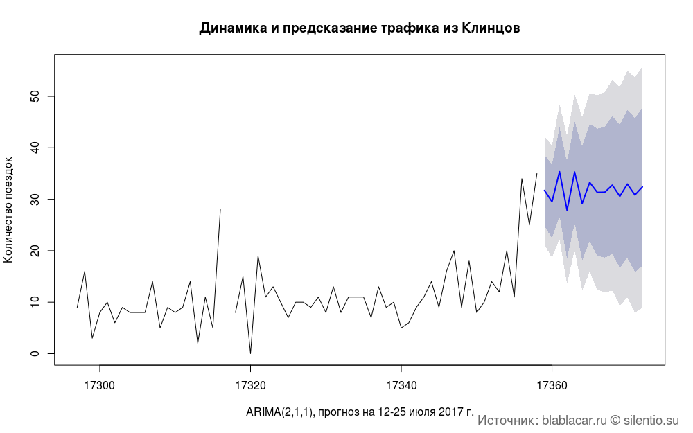
今後1週間または1か月のトラフィックを予測することも問題です。 いくつかのモデルをテストしましたが、予測の精度は低いです。
#### #### bl.arima <- zoo(bl.date$n, bl.date$Date) model.arima <- auto.arima(bl.arima) predic.ar <- forecast(model.arima, h = 14) plot(predic.ar, type = "line", main = " ") title(main = " ", xlab = "ARIMA(2,1,1), 12-25 2017 .", ylab = " ") grid.text(": blablacar.ru silentio.su", x = 0.98, y = 0.02, just = c("right", "bottom"), gp = gpar(fontsize = 14, col = "dimgrey"))
最も人気のある目的地
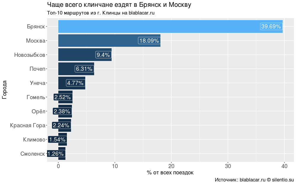
2か月間、Klintsyの車は59の異なる都市に行きました。 ただし、主な方向はほとんどありません:ブリャンスク(全旅行の40%)、モスクワ(18%)、ブリャンスク地方の都市、ホメリ(ベラルーシの境界都市、地域の中心)、オレル、スモレンスク-すべての旅行の88%。
#### #### bl.city <- blblcars %>% count(City) bl.city$percents <- round(bl.city$n/sum(bl.city$n)*100, digits = 2) bl.city <- bl.city %>% arrange(desc(n)) # 59 length(unique(bl.city$City)) #### "-10 . blablacar.ru" #### ggplot(bl.city[1:10,], aes(x = reorder(City, n), y = percents, fill = percents))+ geom_bar(stat = "identity")+ coord_flip()+ geom_label(aes(label = paste0(percents, "%")), size = 5, colour = "white", hjust = 1)+ labs(title = " ", subtitle = "-10 . blablacar.ru", caption = ": blablacar.ru silentio.su", x = "", y = "% ")+ theme(legend.position = "none", axis.text.x = element_text(size = 14), axis.title.x = element_text(size = 14), axis.text.y = element_text(size = 14), axis.title.y = element_text(size = 14), title = element_text(size = 14))
マップ上に目的地を置くと、中心がクリンツィーで半径が1000-1200 kmのほぼ完全な円が得られ、中心は密集し、周辺に放電されます。 Klintsy-Bryansk-Kaluga-Moscow弧もはっきりと見えます。
#### . blablacar.ru #### # bl.city <- na.omit(bl.city) geo <- geocode(bl.city$City) bl.city <- cbind(bl.city, as.data.frame(geo)) map <- get_map(location = "Klintsy", maptype = "terrain", zoom = 4) ggmap(map)+ geom_point(data = bl.city, aes(x = lon, y = lat, size = percents), alpha = 1, colour = "red")+ labs(title = " . blablacar.ru", caption = ": blablacar.ru silentio.su", x = " ", y = " ", size = "% :")+ theme(legend.position = "left", legend.text = element_text(size = 12), axis.text.x = element_text(size = 8), axis.title.x = element_text(size = 8), axis.text.y = element_text(size = 8), axis.title.y = element_text(size = 8), title = element_text(size = 14))
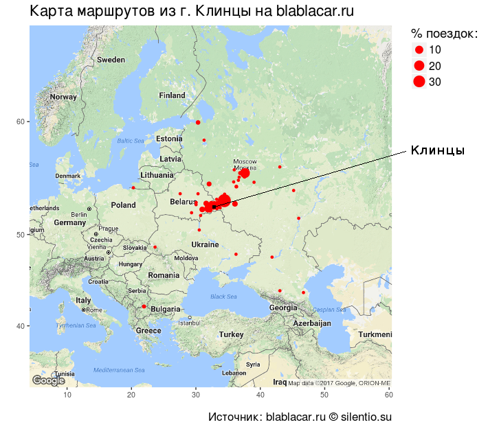
つまり、主に臨床医がその場所を旅行し、近くの地域センターやMSCに定期的に旅行します。
運賃
方向別にグループ化されたすべてのドライバーの運賃はほぼ同じです:約100 p。 -地域では、平均280p。 -ブリャンスク、900 p。 -モスクワ。 これは、通常の航空会社よりも約25%安いです。
価格の最大の変動は、オレル(350から600ルーブル)とスモレンスク(450から650ルーブル)へのチケットです。
#### -10 #### bl.price.top <- blblcars %>% filter(City %in% unique(bl.city$City[1:10])) %>% select(City, Price) bl.price.top <- full_join(bl.price.top, bl.price.top %>% group_by(City) %>% summarise(mean = mean(Price)) ) bl.price.top$mean <- round(bl.price.top$mean, digits = 0) bl.price.top$mean <- paste0(bl.price.top$mean, " .") bl.price.top <- bl.price.top %>% unite(City, c(City, mean), sep = ", ") #### " " #### ggplot(bl.price.top, aes(x = reorder(City, Price), y = Price))+ stat_summary(geom = "line", group = 1, fun.data = "mean_cl_boot", size = 1, colour = "blue")+ stat_summary(fun.data = "mean_cl_boot", colour = "red", size = 1)+ labs(title = " - ", subtitle = " . blablacar.ru (-10 )", caption = ": blablacar.ru silentio.su", x = " ", y = " , .")+ theme(legend.position = "none", legend.text = element_text(size = 14), axis.text.x = element_text(size = 14, angle = 90), axis.title.x = element_text(size = 14), axis.text.y = element_text(size = 14), axis.title.y = element_text(size = 14), title = element_text(size = 14))

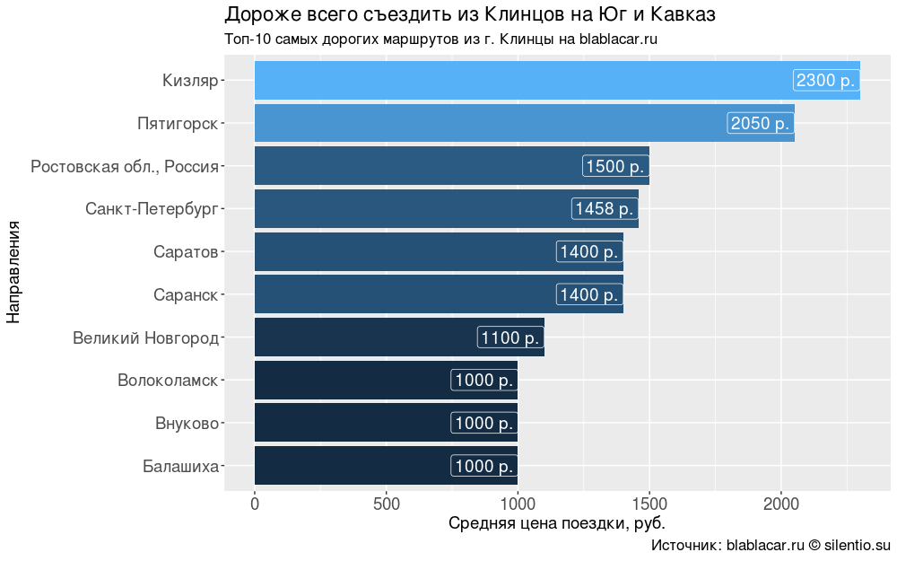
奇妙なことに、旅行の価格は常に距離に依存するとは限りません。 クリンツィーから南とコーカサスへの最も高価な旅行は1500-2300 pです。 ヨーロッパの方向の同様の距離については、彼らは半分を要求します。
#### #### bl.price <- blblcars %>% select(City, Price) %>% group_by(City) %>% summarise(price = mean(Price)) bl.price$price <- round(bl.price$price, digits = 0) bl.price <- bl.price %>% arrange(desc(price)) #### "-10 . blablacar.ru" #### ggplot(bl.price[1:10,], aes(x = reorder(City, price), y = price, fill = price))+ geom_bar(stat = "identity")+ coord_flip()+ geom_label(aes(label = paste0(price, " .")), size = 5, colour = "white", hjust = 1)+ labs(title = " ", subtitle = "-10 . blablacar.ru", caption = ": blablacar.ru silentio.su", x = "", y = " , .")+ theme(legend.position = "none", axis.text.x = element_text(size = 14), axis.title.x = element_text(size = 14), axis.text.y = element_text(size = 14), axis.title.y = element_text(size = 14), title = element_text(size = 14))
ドライバー分析
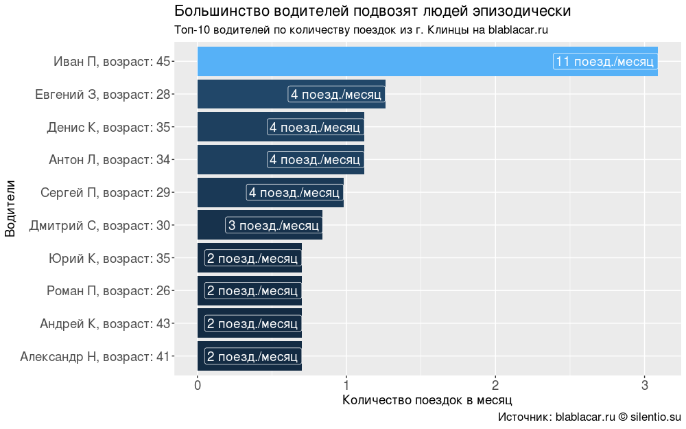
ドライバーのやる気に興味がありました。 なぜ乗客を連れているのですか? 営利目的でこのサービスを使用している人はいますか?
2か月で54%のドライバーがサービスを1回だけ使用しました。 残りは月に1回から週に1回、おそらくビジネス上の問題で移動します。旅行費用を削減するために乗客が連れて行かれます。
私は、たぶん(しかしこれは不正確ですが)商業輸送に従事している人を1人だけ見つけました(ミニバスタクシー、ルート「Novozybkov-Klintsy-Moscow」、3日ごと)。
#### #### drivers <- blblcars %>% select(Name, Age) drivers$Age <- paste0(": ", drivers$Age) drivers <- drivers %>% unite(Name, c(Name, Age), sep = ", ") drivers <- drivers %>% count(Name) drivers$percents <- round(drivers$n/sum(drivers$n)*100, digits = 2) drivers <- arrange(drivers, desc(n)) drivers$per.month <- round(drivers$n/2, digits = 0) summary(as.factor(drivers$n))/sum(drivers$n)*100 #### " " #### ggplot(drivers[1:10,], aes(x = reorder(Name, n), y = percents, fill = percents))+ geom_bar(stat = "identity")+ coord_flip()+ geom_label(aes(label = paste0(per.month, " ./")), size = 5, colour = "white", hjust = 1)+ labs(title = " ", subtitle = "-10 . blablacar.ru", caption = ": blablacar.ru silentio.su", x = "", y = " ")+ theme(legend.position = "none", axis.text.x = element_text(size = 14), axis.title.x = element_text(size = 14), axis.text.y = element_text(size = 14), axis.title.y = element_text(size = 14), title = element_text(size = 14))
出発時間
Klintsyを16:00〜19:00に出発するのが最も簡単です。 車は夜9時、夜にモスクワに行きます。
#### -10 #### bl.hours <- blblcars %>% group_by(City) %>% count(hours) bl.hours <- ungroup(bl.hours) # for (i in unique(bl.hours$City)) { for (j in seq(0, 23, 1)) { if (!j %in% bl.hours$hours[bl.hours$City == i]) { bl.hours <- rbind(bl.hours, data.frame(City = i, hours = j, n = 0)) } } } # -10 bl.hours <- bl.hours %>% filter(City %in% bl.city$City[1:10]) bl.hours$percents <- round(bl.hours$n/sum(bl.hours$n)*100, digits = 2) #### " . blablacar.ru " #### ggplot(bl.hours, aes(x = hours, y = percents, fill = City))+ geom_bar(stat = "identity")+ labs(title = " 16:00 19:00", subtitle = " . blablacar.ru ", caption = ": blablacar.ru silentio.su", x = " ( )", y = "% ( -10)", fill = ":")+ theme(legend.position = "right", legend.text = element_text(size = 12), axis.text.x = element_text(size = 14), axis.title.x = element_text(size = 14), axis.text.y = element_text(size = 14), axis.title.y = element_text(size = 14), title = element_text(size = 14))

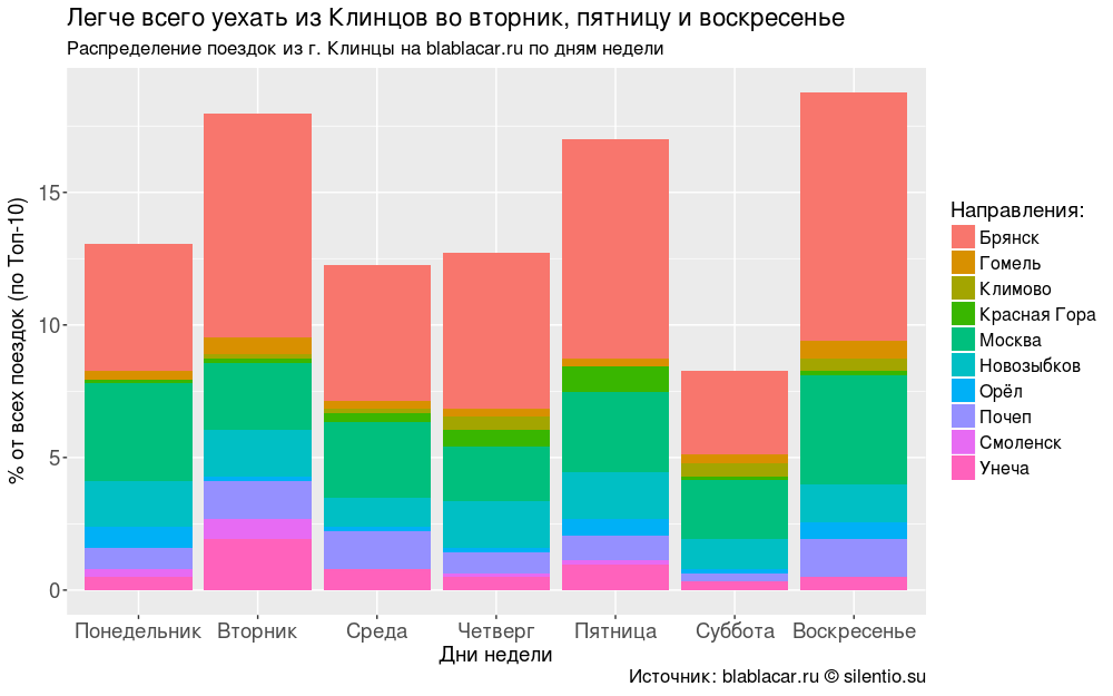
ほとんどの場合、人々は火曜日、金曜日、日曜日に街を離れます。
#### -10 #### bl.days <- blblcars %>% group_by(City) %>% count(days) bl.days <- ungroup(bl.days) # for (i in unique(bl.days$City)) { for (j in unique(bl.days$days)) { if (!j %in% bl.days$days[bl.days$City == i]) { bl.days <- rbind(bl.days, data.frame(City = i, days = j, n = 0)) } } } # -10 bl.days <- bl.days %>% filter(City %in% bl.city$City[1:10]) bl.days$percents <- round(bl.days$n/sum(bl.days$n)*100, digits = 2) # bl.days$days <- as.factor(bl.days$days) bl.days$days <- factor(bl.days$days, levels = c("", "", "", "", "", "", "")) #### " . blablacar.ru " #### ggplot(bl.days, aes(x = days, y = percents, fill = City))+ geom_bar(stat = "identity")+ labs(title = " , ", subtitle = " . blablacar.ru ", caption = ": blablacar.ru silentio.su", x = " ", y = "% ( -10)", fill = ":")+ theme(legend.position = "right", legend.text = element_text(size = 12), axis.text.x = element_text(size = 14), axis.title.x = element_text(size = 14), axis.text.y = element_text(size = 14), axis.title.y = element_text(size = 14), title = element_text(size = 14))
おわりに
研究の結果に基づいて、そのような欲求があればどこに、いつ、どのくらい行く可能性が高いかを説明するスケジュールをまとめました。
#### #### tbls <- blblcars %>% filter(City %in% bl.city$City[1:10]) %>% group_by(City) %>% select(City, days, Time, Price) # tbls <- full_join(tbls, tbls %>% summarise(mean.price = round(mean(Price), digits = 0)), by = "City" ) tbls <- tbls %>% select(-Price) # tbls <- full_join(tbls, tbls %>% count(days) %>% top_n(1, n), by = "City") for (i in unique(tbls$City)) { tbls$days.y[tbls$City == i] <- paste0(unique(tbls$days.y[tbls$City == i]), collapse = ", ") } tbls <- tbls %>% select(-c(days.x, n)) # tbls <- full_join(tbls, tbls %>% count(Time) %>% top_n(1, n), by = "City") for (i in unique(tbls$City)) { tbls$Time.y[tbls$City == i] <- paste0(unique(tbls$Time.y[tbls$City == i]), collapse = ", ") } tbls <- tbls %>% select(-c(Time.x, n)) tbls <- ungroup(tbls) tbls <- unique(tbls) tbls <- tbls[c("City", "days.y", "Time.y", "mean.price")] colnames(tbls) <- c(" ", " ", " ", " ") tbls <- tbls %>% arrange(` `) write.csv(tbls, file = "data/tbls.csv", row.names = F)

また、曜日と出発時刻に基づいて最も可能性の高いルートを予測するxgboostアルゴリズムをトレーニングしました。
最も有益な兆候は出発時間でした。 夜遅く、モデルは一貫して、午後にノボジブコフに、夜にブリャンスクに、モスクワに行くことを勧めます。 他の都市への旅行xgboostはほとんどありません。
#### XGBOOST #### # df <- read.csv("data/ - .csv", stringsAsFactors = F) df <- df %>% select(c(City, Time, days)) df <- df %>% separate(Time, c("hours", "minutes"), sep = ":") df$days <- as.factor(df$days) levels(df$days) <- c("7", "2", "1", "5", "3", "6", "4") df[,2:4] <- apply(df[,2:4], 2, function(x) as.numeric(x)) top10 <- df %>% count(City) %>% arrange(desc(n)) top10 <- top10$City[1:10] df <- df %>% filter(City %in% top10) df <- na.omit(df) # df$class <- as.numeric(as.factor(df$City))-1 City.class <- df %>% select(City, class) City.class <- unique(City.class) df <- df[,-1] # train test # 1/3 indexes <- createDataPartition(df$class, times = 1, p = 0.7, list = F) train <- df[indexes,] test <- df[-indexes,] # y.train <- train$class # train.m <- data.matrix(train[,-4]) train.m <- xgb.DMatrix(train.m, label = y.train) # Stopping. Best iteration: # [15] train-merror:0.425361+0.010171 # test-merror:0.504626+0.035449 model <- xgb.cv(data = train.m, nfold = 4, eta = 0.03, nrounds = 2000, num_class = 10, objective = "multi:softmax", early_stopping_round = 200) # # train$class <- as.factor(train$class) traintask <- makeClassifTask(data = train, target = "class") lrn <- makeLearner("classif.xgboost", predict.type = "response") lrn$par.vals <- list(objective = "multi:softmax", eval_metric = "merror", nrounds = 15, eta = 0.03) params <- makeParamSet(makeDiscreteParam("booster", values = c("gbtree", "gblinear")), makeIntegerParam("max_depth", lower = 1, upper = 10), makeNumericParam("min_child_weight", lower = 1, upper = 10), makeNumericParam("subsample", lower = 0.5, upper = 1), makeNumericParam("colsample_bytree", lower = 0.5, upper = 1)) rdesc <- makeResampleDesc("CV", iters = 4) # ctrl <- makeTuneControlRandom(maxit = 10) # mytune <- tuneParams(learner = lrn, task = traintask, resampling = rdesc, par.set = params, control = ctrl, show.info = T) # [Tune-y] 10: mmce.test.mean=0.525; time: 0.0 min # [Tune] Result: booster=gbtree; max_depth=10; min_child_weight=5; # subsample=0.99; colsample_bytree=0.907 : mmce.test.mean=0.516 # Xgboost-model # param <- list( "num_class" = 10, "objective" = "multi:softmax", "eval_metric" = "merror", "eta" = 0.03, "max_depth" = 10, "min_child_weight" = 5, "subsample" = 0.99, "colsample_bytree" = 0.907) # model <- xgb.cv(data = train.m, params = param, nfold = 4, nrounds = 20000, early_stopping_round = 100) # Stopping. Best iteration: # [84] train-merror:0.462308+0.015107 test-merror:0.509050+0.028020 # Xgboost- model <- xgboost(data = train.m, params = param, nrounds = 84, scale_pos_weight = 5) # test-matrix y.test <- test$class test <- data.matrix(test[,-4]) # mat <- xgb.importance(feature_names = colnames(train.m), model = model) xgb.plot.importance(importance_matrix = mat, main = " :") # y.predict <- predict(model, test, nrounds = 84, scale_pos_weight = 5) # replace.class <- function(x){ for (i in unique(x)) { x[x == i] <- City.class$City[City.class$class == i] } return(x) } # confusionMatrix(replace.class(y.predict), replace.class(y.test)) # # df_test <- data.frame(hours = as.numeric(sample(x = c(0:23), size = 10, replace = T)), minutes = as.numeric(sample(x = c(0:59), size = 10, replace = T)), days = as.numeric(sample(x = c(1:7), size = 10, replace = T))) # df_test$City <- replace.class(predict(model, data.matrix(df_test), nrounds = 84, scale_pos_weight = 5)) # df_test <- df_test[c("City", "days", "hours", "minutes")] colnames(df_test) <- c(" ", " ", " ", " ") df_test <- df_test %>% arrange(` `) grid.text(" xgboost", x = 0.5, y = 0.93, just = c("centre", "bottom"), gp = gpar(fontsize = 16)) grid.table(df_test) grid.text(": blablacar.ru", x = 0.02, y = 0.01, just = c("left", "bottom"), gp = gpar(fontsize = 11)) grid.text(" silentio.su", x = 0.98, y = 0.01, just = c("right", "bottom"), gp = gpar(fontsize = 11))

見出しで提示された質問に答えると、答えは「はい、Klintsyから離れることができます。 近いだけ これはオムスクではありません。」