初心者向け人工ニューラルネットワークの数学、パート2-勾配降下

パート1-線形回帰



最初の部分で、ランダムに生成されたデータが自分の好みに合わない場合は、ここから適切な例を取り上げることができません。 あなたはオタク 、 ワインメーカー 、 セラーのように感じることができます。 そして、これらすべては椅子から立ち上がることなく行われます。 多くのデータセットと1つの条件があります。公開時には、他の人が結果を再現できるように、データの出所を示します。

勾配降下

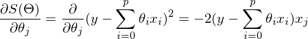
最後の部分では、最小二乗法を使用して線形回帰パラメーターを計算する例を示しました。 パラメータが分析的に見つかりました- どこで 擬似逆行列です。 このソリューションは、明確で正確かつ短いものです。 しかし、数値的に解決できる問題があります。 勾配降下法は、ニューラルネットワーク、SVM、k-means、回帰など、関数の極値を見つける必要がある多くのアルゴリズムで使用できる数値最適化の方法です。 ただし、純粋な形で知覚する方が簡単です（変更する方が簡単です）。



問題は、疑似逆行列の計算が非常に高価であるということです 。 、逆行列を見つける- 行列ベクトル乗算 ここで、nはマトリックスAの要素数（属性の数*テストサンプルの要素数）です。マトリックスAの要素数が大きい場合（> 10 ^ 6-など）、10,000のコアがある場合でも、解析は遅延する可能性があります。 また、一次導関数は非線形になり、解が複雑になるか、分析解がまったくないか、データがメモリに収まらず、反復アルゴリズムが必要になる場合があります。 彼らはプラスと数値解が完全に正確ではないという事実を書き留めることが起こります。 この点で、コスト関数は数値的手法によって最小化されます。 極値を見つける問題は、最適化問題と呼ばれます。 このパートでは、勾配降下法と呼ばれる最適化方法に焦点を当てます。



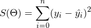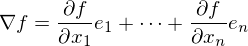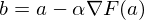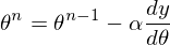
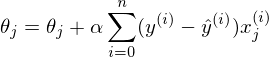
線形回帰とOLSから離れず、損失関数を示します どうやって -彼女は変わりませんでした。 勾配は次の形式のベクトルであることを思い出させてください どこで プライベートデリバティブです。 勾配の特性の1つは、関数fが最も増加する方向を示すことです。 これの証明は、デリバティブの定義から得られます。 いくつかの証拠 。 点aを取ります-この点の近くで、関数Fを定義して微分可能にしなければなりません。逆勾配ベクトルは、関数Fが最も急速に減少する方向を示します。 このことから、ある時点でbと等しいと結論付けます。 、いくつかの小さな 関数の値は、ポイントaの値以下になります。 これは丘を下って移動するものと想像できます。一歩下がったら、現在の位置は前の位置よりも低くなります。 したがって、次の各ステップで、高さは少なくとも増加しません。 正式な定義 。 これらの定義に基づいて、未知のパラメーターを見つけるための式を取得できます（これは上記の式の単なる書き換えバージョンです）。







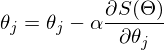メソッドのステップです。 機械学習タスクでは、学習速度と呼ばれます。



この方法は非常にシンプルで直感的で、簡単な2次元の例を使用して説明します。



フォームの機能を最小化する必要があります 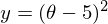。 最小化するとは、どの値で見つけるかを意味します 機能 最小値を取ります。 アクションのシーケンスを定義します。



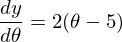
1）に関するデリバティブ ：

2）初期値を設定する = 0

3）ステップサイズを設定します-いくつかの値（0.1、0.9、1.2）を試して、この選択が収束にどのように影響するかを確認します。

4）25回連続で上記の式を満たします。 不明なパラメーターは1つだけなので、式は1つだけです。



コードは非常に簡単です。 関数の定義を除くと、アルゴリズム全体は3行に収まります。







プロセス全体を次のように視覚化できます（青い点は前のステップの値、赤い点は現在の値です）。







または、異なるサイズのステップの場合：







値が1.2の場合、メソッドは分岐し、各ステップは低くならず、むしろ高くなり、無限に急ぎます。 単純な実装のステップは手動で選択され、そのサイズはデータに依存します-勾配が大きく、0.0001のいくつかの異常な値では、不一致が生じる可能性があります。







「悪い」関数を使用した別の例を次に示します。 最初のアニメーションでは、方法も分岐し、高すぎるステップのために長い間丘をさまよいます。 2番目のケースでは、ローカルミニマムが見つかりました。速度値を変えると、グローバルミニマムを見つける方法が見つかりません。 この事実は、この方法の欠点の1つです。関数が凸で滑らかな場合にのみ、グローバルな最小値を見つけることができます。 または、初期値が幸運なら。







また、3次元グラフでアルゴリズムの動作を考慮することもできます。 多くの場合、図の輪郭のみが描かれます。 私は単純な回転放物面を取りました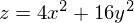： 。 3Dでは、次のようになります。 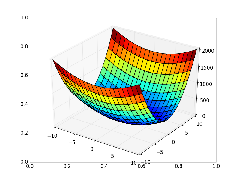、等高線付きのグラフは「上面図」です。











また、すべての勾配線が輪郭に垂直であることに注意してください。 これは、反勾配に向かって移動すると、1ステップで最小値にすぐにジャンプすることができないことを意味します-勾配はそこにまったくないことを示します。



グラフィックの説明の後、未知のパラメーターを計算するための式を見つけます OLSを使用した線形回帰。







テストサンプルの要素数が1に等しい場合、式はそのままにしてカウントできます。 要素がn個ある場合、アルゴリズムは次のようになります。



v回繰り返す

{



jごとに同時に。

}、nはトレーニングセットの要素数、vは反復回数



同時性の要件は、シータの古い値で導関数を計算する必要があることを意味します。最初のパラメーターを個別に計算し、次に2番目などを計算する必要はありません。最初のパラメーターを個別に変更した後、導関数はその値も変更するためです 同時変更の擬似コード：

 for i in train_samples: new_theta[1] = old_theta[1] + a * derivative(old_theta) new_theta[2] = old_theta[2] + a * derivative(old_theta) old_theta = new_theta
      
      

        
        
        
      

    
        
        
        
      
      

        
        
        
      

    
     

パラメータ値を個別に計算する場合、これは勾配降下ではありません。 3次元の図形があり、パラメーターを1つずつ計算すると、このプロセスが一度に1つの座標だけを移動することを想像できます-x座標に沿って1ステップ、次にy座標に沿ったステップなど。 反勾配ベクトルに向かって移動する代わりに、ステップ。



上記のアルゴリズムのバージョンは、バースト勾配降下法と呼ばれます。 繰り返し回数は、「収束するまで繰り返す」というフレーズに置き換えることができます。 このフレーズは、コスト関数の以前の値と現在の値が等しくなるまでパラメーターが調整されることを意味します。 これは、ローカルまたはグローバルの最小値が検出されたことを意味し、アルゴリズムはそれ以上進みません。 実際には、平等は達成できず、収束の限界が導入されます 。 これは小さな値で確立され、停止基準は、以前の値と現在の値の差が収束限界よりも小さいことです。これは、目的の確立された精度で最小値に達することを意味します。 より高い精度（より少ない ）-アルゴリズムの反復。 次のようになります。

 while abs(S_current - S_previous) >= Epsilon: # do something
      
      

        
        
        
      

    
        
        
        
      
      

        
        
        
      

    
     

投稿が突然伸びたので、これで終了したいと思います。次のパートでは、OLSを使用した線形回帰の勾配降下の分析を続けます。



継続する 。



例を実行するには、numpy、matplotlibが必要です。

ImageMagickは、アニメーションアニメーションの例を実行するために必要です。

記事で使用されている資料-github.com/m9psy/neural_network_habr_guide