この記事では、センチメントセンチメントの単純な分析を行う方法を示します。 特定のトピックに関するtwitterメッセージをアップロードし、ポジティブな単語とネガティブな単語のデータベースと比較します。 見つかった正と負の単語の比率は、調性の比率と呼ばれます。 また、最も一般的な単語を見つけるための関数も作成します。 これらの言葉は、世論や感情に関する有用な文脈情報を提供できます。 意見を表すポジティブな単語とネガティブな単語のデータセット(調子のある単語)は、 Hugh and Lew、KDD-2004から取得したものです。
twitteR, dplyr, stringr, ggplot2, tm, SnowballC, qdap
、
wordcloud
を使用したR実装。 使用する前に、
install.packages()
および
library()
コマンドを使用してこれらのパッケージをインストールおよびダウンロードする必要があります。
Twitter APIをダウンロードする
最初のステップは、開発者ポータルでTwitterに登録し、承認を受けることです。 あなたが必要になります:
api_key = " API" api_secret = " api_secret " access_token = " " access_token_secret = " "
このデータを受け取ったら、ログインしてTwitter APIにアクセスします。
setup_twitter_oauth(api_key,api_secret,access_token,access_token_secret)
辞書をダウンロードする
次のステップは、正と負の音調の単語(辞書)の配列を作業フォルダーRにロードすることです。以下に示すように、変数
positive
と
negative
から単語を抽出できます。
positive=scan('positive-words.txt',what='character',comment.char=';') negative=scan('negative-words.txt',what='character',comment.char=';') positive[20:30]
## [1] "accurately" "achievable" "achievement" "achievements" ## [5] "achievible" "acumen" "adaptable" "adaptive" ## [9] "adequate" "adjustable" "admirable"
negative[500:510]
## [1] "byzantine" "cackle" "calamities" "calamitous" ## [5] "calamitously" "calamity" "callous" "calumniate" ## [9] "calumniation" "calumnies" "calumnious"
合計2006の肯定的な単語と4783の否定的な単語。 上記のセクションでは、これらの辞書の単語の例をいくつか示しています。
辞書に新しい単語を追加したり、既存の単語を削除したりできます。 以下のコードを使用して、ワード
cloud
を
positive
辞書に追加し、
negative
辞書から削除します。
positive=c(positive,"cloud") negative=negative[negative!="cloud"]
Twitter投稿検索
次のステップでは、twitterメッセージの検索文字列を設定し、その値を変数
findfd
ます。 分析に使用されるツイートの数は、別の変数
number
割り当てられます。 メッセージの検索と情報の取得にかかる時間は、この数値によって異なります。 遅いインターネット接続または複雑な検索クエリは、遅延を引き起こす可能性があります。
findfd= "CyberSecurity" number= 5000
上記のコードでは、文字列「CyberSecurity」と5000件のツイートを使用しています。 Twitter検索コード:
tweet=searchTwitter(findfd,number)
## Time difference of 1.301408 mins
ツイートテキストの取得
ツイートには多くの追加フィールドとシステム情報があります。
gettext()
関数を使用してテキストフィールドを取得し、結果のリストを
tweetT
変数に
tweetT
ます。 この機能は、5000件のツイートすべてに適用されます。 以下のコードは、最初の5つのメッセージのサンプリング結果も示しています。
tweetT=lapply(tweet,function(t)t$getText()) head(tweetT,5)
## [[1]] ## [1] "RT @PCIAA: \"You must have realtime technology\" how do you defend against #Cyberattacks? @FireEye #cybersecurity http://t.co/Eg5H9UmVlY" ## ## [[2]] ## [1] "@MPBorman: '#Cybersecurity on agenda for 80% corporate boards http://t.co/eLfxkgi2FT @CS… http://t.co/h9tjop0ete http://t.co/qiyfP94FlQ" ## ## [[3]] ## [1] "The FDA takes steps to strengthen cybersecurity of medical devices | @scoopit via @60601Testing http://t.co/9eC5LhGgBa" ## ## [[4]] ## [1] "Senior Solutions Architect, Cybersecurity, NYC-Long Island region, Virtual offic... http://t.co/68aOUMNgqy #job#cybersecurity" ## ## [[5]] ## [1] "RT @Cyveillance: http://t.co/Ym8WZXX55t #cybersecurity #infosec - The #DarkWeb As You Know It Is A Myth via @Wired http://t.co/R67Nh6Ck70"
テキストクリア機能
このステップでは、一連のコマンドを実行してテキストをクリアする関数を作成します。句読点、特殊文字、リンク、余分なスペース、数字を削除します。 この関数は、
tolower()
を使用して大文字を小文字にキャストします。
tolower()
関数は、特殊文字に遭遇した場合にエラーをスローすることが多く、コードの実行は停止します。 これを防ぐために、エラーを
tryTolower
する関数
tryTolower
作成し、テキスト消去関数のコードで使用します。
tryTolower = function(x) { y = NA # tryCatch error try_error = tryCatch(tolower(x), error = function(e) e) # if not an error if (!inherits(try_error, "error")) y = tolower(x) return(y) }
clean()関数は、ツイートをクリーンアップし、文字列を単語ベクトルに分割します。
clean=function(t){ t=gsub('[[:punct:]]','',t) t=gsub('[[:cntrl:]]','',t) t=gsub('\\d+','',t) t=gsub('[[:digit:]]','',t) t=gsub('@\\w+','',t) t=gsub('http\\w+','',t) t=gsub("^\\s+|\\s+$", "", t) t=sapply(t,function(x) tryTolower(x)) t=str_split(t," ") t=unlist(t) return(t) }
ツイートをクリアして単語に分割する
このステップでは、
clean()
関数を使用して5000のツイートをクリアします。 結果は
tweetclean
リスト
tweetclean
保存され
tweetclean
。 次のコードは、この関数を使用して、最初の5つのツイートを剥がして単語に分割することも示しています。
tweetclean=lapply(tweetT,function(x) clean(x)) head(tweetclean,5)
## [[1]] ## [1] "rt" "pciaa" "you" "must" ## [5] "have" "realtime" "technology" "how" ## [9] "do" "you" "defend" "against" ## [13] "cyberattacks" "fireeye" "cybersecurity" ## ## [[2]] ## [1] "mpborman" "cybersecurity" "on" "agenda" ## [5] "for" "" "corporate" "boards" ## [9] " " "cs" ## ## [[3]] ## [1] "the" "fda" "takes" "steps" ## [5] "to" "strengthen" "cybersecurity" "of" ## [9] "medical" "devices" "" "scoopit" ## [13] "via" "testing" ## ## [[4]] ## [1] "senior" "solutions" "architect" ## [4] "cybersecurity" "nyclong" "island" ## [7] "region" "virtual" "offic" ## [10] "" "jobcybersecurity" ## ## [[5]] ## [1] "rt" "cyveillance" "" "cybersecurity" ## [5] "infosec" "" "the" "darkweb" ## [9] "as" "you" "know" "it" ## [13] "is" "a" "myth" "via" ## [17] "wired"
ツイート分析
ツイート分析の実際のタスクに到達しました。 ツイートのテキストと辞書を比較し、一致する単語を見つけます。 これを行うために、データベースからの単語と一致する正と負の単語をカウントする関数を最初に定義します。 以下は、正の一致をカウントするための
returnpscore
関数
returnpscore
です。
returnpscore=function(tweet) { pos.match=match(tweet,positive) pos.match=!is.na(pos.match) pos.score=sum(pos.match) return(pos.score) }
次に、関数を
tweetclean
リストに適用します。
positive.score=lapply(tweetclean,function(x) returnpscore(x))
次のステップは、ツイート内の肯定的な単語の総数をカウントするループを設定することです。
pcount=0 for (i in 1:length(positive.score)) { pcount=pcount+positive.score[[i]] } pcount
## [1] 1569
上記のように、ツイートには1569の肯定的な単語があります。 同様に、負の数を見つけることができます。 以下のコードは、正と負の発生を考慮しています。
poswords=function(tweets){ pmatch=match(t,positive) posw=positive[pmatch] posw=posw[!is.na(posw)] return(posw) }
この関数は
tweetclean
リストに適用され、ループ内の単語はデータフレーム
pdatamart
追加されます。 以下のコードは、ポジティブワードの最初の10個の出現を示しています。
words=NULL pdatamart=data.frame(words) for (t in tweetclean) { pdatamart=c(poswords(t),pdatamart) } head(pdatamart,10)
## [[1]] ## [1] "best" ## ## [[2]] ## [1] "safe" ## ## [[3]] ## [1] "capable" ## ## [[4]] ## [1] "tough" ## ## [[5]] ## [1] "fortune" ## ## [[6]] ## [1] "excited" ## ## [[7]] ## [1] "kudos" ## ## [[8]] ## [1] "appropriate" ## ## [[9]] ## [1] "humour" ## ## [[10]] ## [1] "worth"
同様に、負の調子の単語をカウントするための多くの関数とループが作成されます。 この情報は、別のデータフレーム
ndatamart
ます。 以下は、ツイートの最初の10個の否定的な単語のリストです。
head(ndatamart,10)
## [[1]] ## [1] "attacks" ## ## [[2]] ## [1] "breach" ## ## [[3]] ## [1] "issues" ## ## [[4]] ## [1] "attacks" ## ## [[5]] ## [1] "poverty" ## ## [[6]] ## [1] "attacks" ## ## [[7]] ## [1] "dead" ## ## [[8]] ## [1] "dead" ## ## [[9]] ## [1] "dead" ## ## [[10]] ## [1] "dead"
一般的なネガティブおよびポジティブな単語のチャート
このセクションでは、いくつかのグラフを作成して、頻繁に発生する否定語と肯定語の分布を示します。
unlist()
関数を使用して、リストをベクトルに変換します。 ベクトル変数
pwords
および
nwords
は、データフレームオブジェクトに
nwords
れます。
dpwords=data.frame(table(pwords)) dnwords=data.frame(table(nwords))
dplyr
パッケージを使用して
dplyr
単語を文字型の変数に
dplyr
から、発生
frequency > 15
(
frequency > 15
)で正と負
dplyr
単語を
dplyr
必要があります。
dpwords=dpwords%>% mutate(pwords=as.character(pwords))%>% filter(Freq>15)
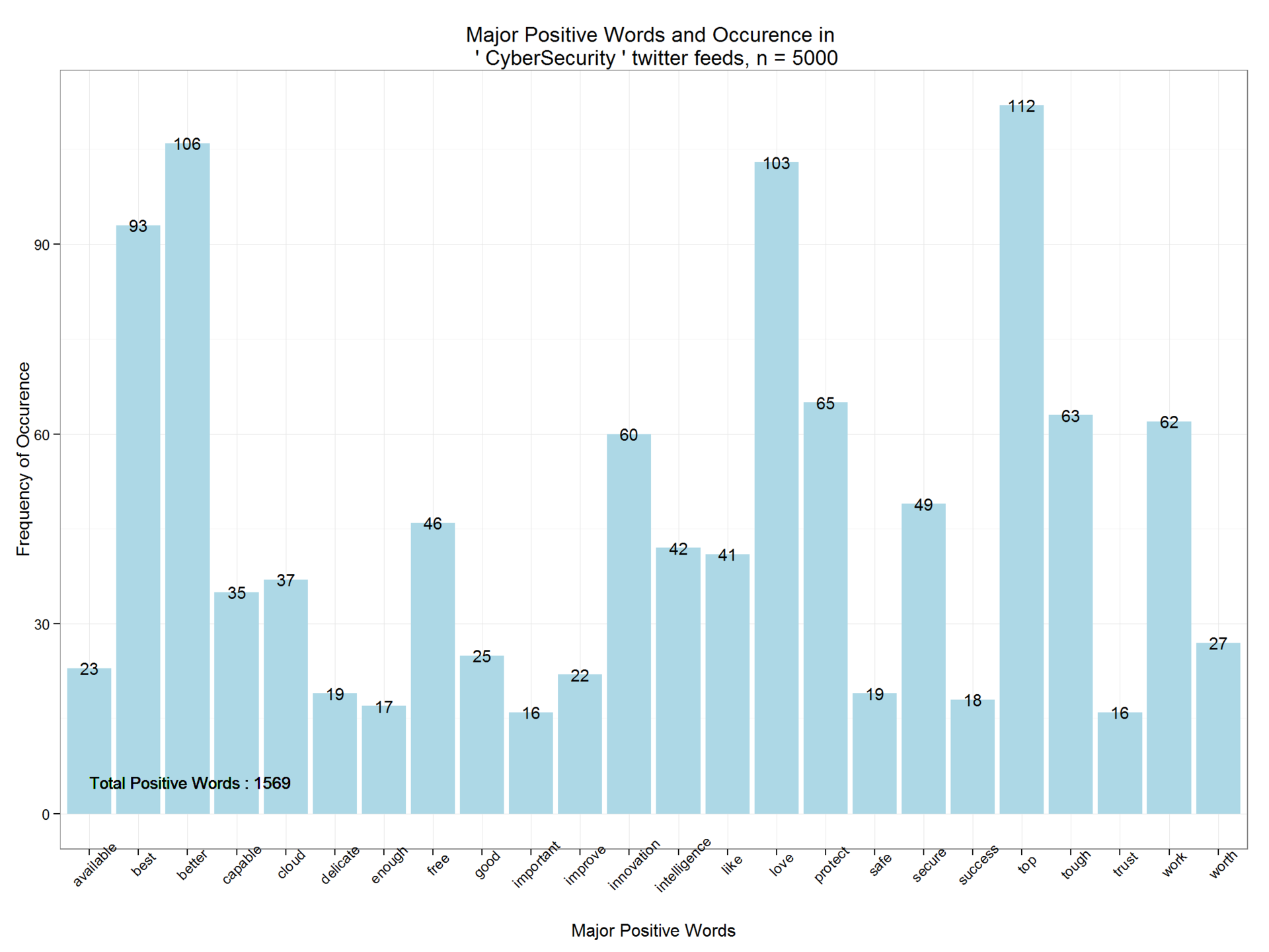
ggplot2
パッケージを使用して、主要なポジティブワードとその頻度を
ggplot2
ます。 ご覧のとおり、ポジティブワードは1569のみで、分布関数はポジティブな調性の度合いを示しています。
ggplot(dpwords,aes(pwords,Freq))+geom_bar(stat="identity",fill="lightblue")+theme_bw()+ geom_text(aes(pwords,Freq,label=Freq),size=4)+ labs(x="Major Positive Words", y="Frequency of Occurence",title=paste("Major Positive Words and Occurence in \n '",findfd,"' twitter feeds, n =",number))+ geom_text(aes(1,5,label=paste("Total Positive Words :",pcount)),size=4,hjust=0)+theme(axis.text.x=element_text(angle=45))
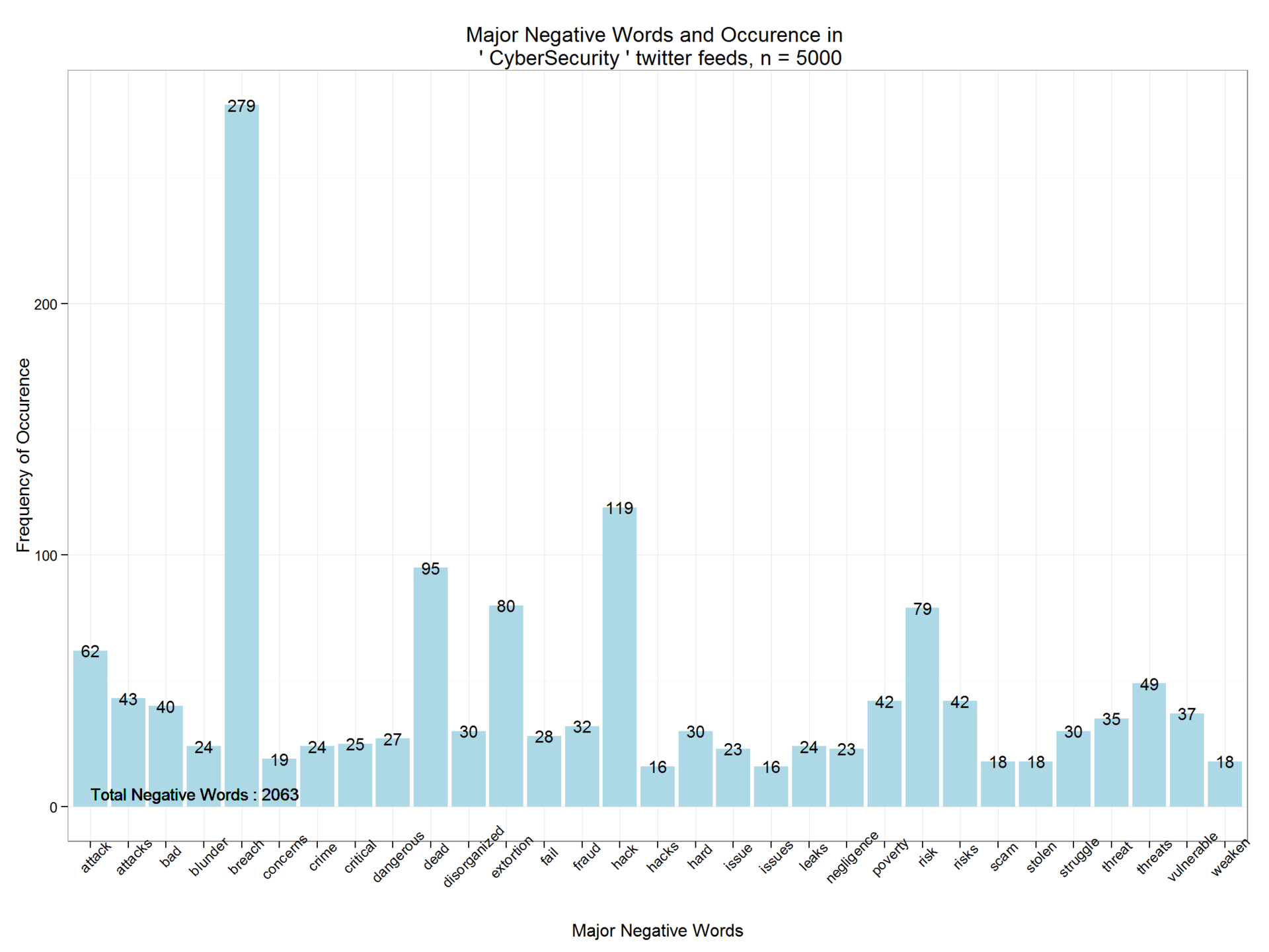
同様に、否定語とその頻度を推測します。 CyberSecurity検索文字列を含む5,000件のツイートには、2,063個の否定的な単語が含まれています。
一般的な単語を削除して、ワードクラウドを作成する
VectorSource
関数を使用して、
VectorSource
を単語のブロックに
VectorSource
ます。 ブロックの形式で表現すると、テキストマイニングパッケージ
tm
を使用して、冗長な一般的な単語を削除できます。 いわゆるストップワードと呼ばれる一般的な単語を削除することで、重要かつ強調されたコンテキストに集中することができます。 以下のコードは、ストップワードの例を示しています。
tweetscorpus=Corpus(VectorSource(tweetclean)) tweetscorpus=tm_map(tweetscorpus,removeWords,stopwords("english")) stopwords("english")[30:50]
## [1] "what" "which" "who" "whom" "this" "that" "these" ## [8] "those" "am" "is" "are" "was" "were" "be" ## [15] "been" "being" "have" "has" "had" "having" "do"
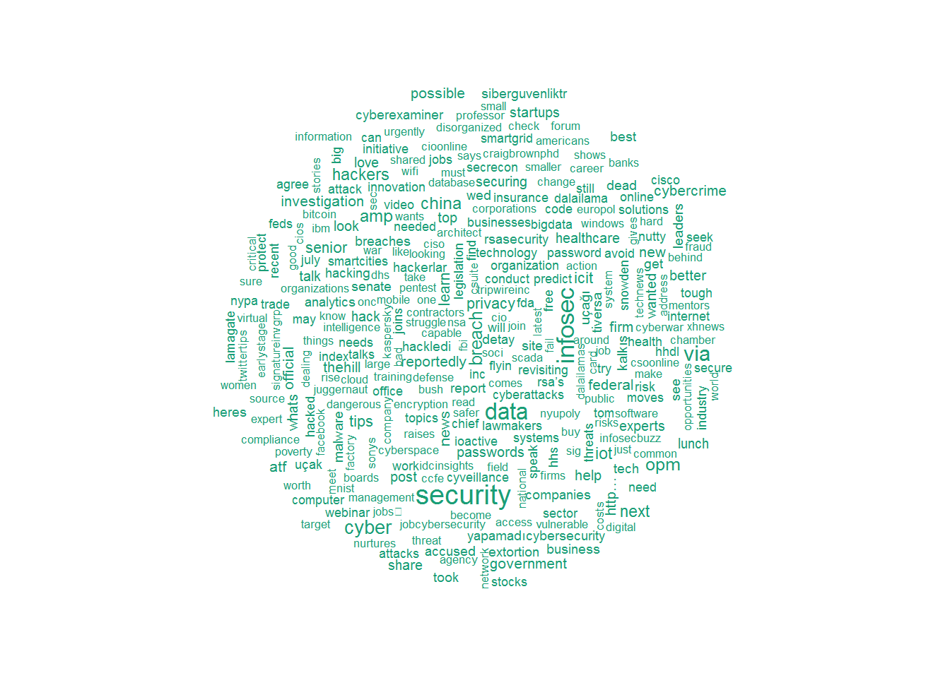
wordcloud
パッケージを使用して、ツイート用のワードクラウドを作成します。 最大数量は300に制限されていることに注意してください。
wordcloud(tweetscorpus,scale=c(5,0.5),random.order = TRUE,rot.per = 0.20,use.r.layout = FALSE,colors = brewer.pal(6,"Dark2"),max.words = 300)
一般的な単語の分析とグラフ化
この最後の手順では、
DocumentTermMatrix
関数を使用して、単語のブロックをドキュメントのマトリックスに変換します。 頻繁に発生する非定型単語について、ドキュメントのマトリックスを分析できます。 次に、ブロックからまれな単語を削除します(出現頻度が低すぎます)。 以下のコードは、最も一般的なもの(頻度50以上)を表示します。
dtm=DocumentTermMatrix(tweetscorpus) # #removing sparse terms dtms=removeSparseTerms(dtm,.99) freq=sort(colSums(as.matrix(dtm)),decreasing=TRUE) #get some more frequent terms findFreqTerms(dtm,lowfreq=100)
## [1] "amp" "atf" "better" "breach" ## [5] "china" "cyber" "cybercrime" "cybersecurity" ## [9] "data" "experts" "federal" "firm" ## [13] "government" "hackers" "hack" "healthcare" ## [17] "help" "heres" "http…" "icit" ## [21] "infosec" "investigation" "iot" "learn" ## [25] "look" "love" "lunch" "new" ## [29] "news" "next" "official" "opm" ## [33] "passwords" "possible" "post" "privacy" ## [37] "reportedly" "securing" "security" "senior" ## [41] "share" "site" "startups" "talk" ## [45] "thehill" "tips" "took" "top" ## [49] "via" "wanted" "wed" "whats"
最後に、マトリックスをデータフレームに移動し、
Minimum frequency > 75
でフィルター処理し、
ggplot2
を使用してグラフをプロットします。
wf=data.frame(word=names(freq),freq=freq) wfh=wf%>% filter(freq>=75,!word==tolower(findfd))
ggplot(wfh,aes(word,freq))+geom_bar(stat="identity",fill='lightblue')+theme_bw()+ theme(axis.text.x=element_text(angle=45,hjust=1))+ geom_text(aes(word,freq,label=freq),size=4)+labs(x="High Frequency Words ",y="Number of Occurences", title=paste("High Frequency Words and Occurence in \n '",findfd,"' twitter feeds, n =",number))+ geom_text(aes(1,max(freq)-100,label=paste("# Positive Words:",pcount,"\n","# Negative Words:",ncount,"\n",result(ncount,pcount))),size=5, hjust=0)
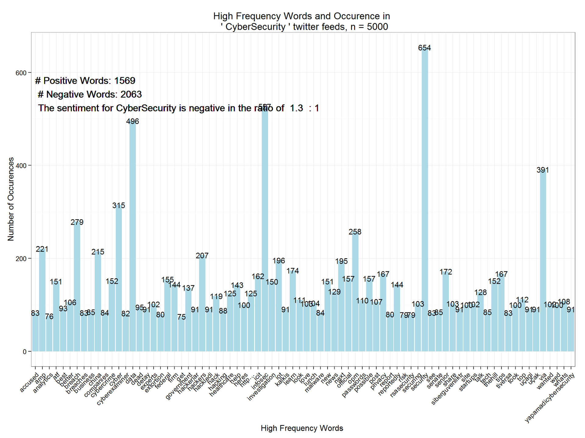
結論
ご覧のとおり、CyberSecurityの調性は1.3の比率で負です。1.この分析は、傾向を強調するために、いくつかの時間間隔で拡張できます。 また、関連するトピックで反復的に実装して、相対的な調性評価を比較および分析することもできます。