特大のPostgres

たまたま、最近、さまざまなシステムの最適化とスケーリングに対処しなければなりませんでした。 タスクの1つはPostgreSQLのスケーリングでした。 データベースの最適化は通常どのように行われますか？ おそらく最初に検討するのは、ジョブに最適な設定を選択する方法と、作成できるインデックスです。 少しでもうまくいかない場合は、サーバーの容量を増やし、ログファイルを別のディスクに転送し、負荷を分散し、テーブルをパーティション分割し、あらゆる種類のモデルをリファクタリングおよび再設計します。 そして今、すべてが完全に調整されていますが、これらすべての体の動きが十分ではない時が来ます。 次に何をする？ 水平スケーリングとデータシャーディング。







水平方向にスケーラブルなクラスターをPostgres-XL DBMSにデプロイした経験を共有したいと思います。



Postgres-XLは、単一のデータベースインスタンスとして機能するように複数のPostgreSQLクラスターを組み合わせることができる優れたツールです。 データベースに接続するクライアントに違いはなく、単一のPostgreSQLインスタンスまたはPostgres-XLクラスターで動作します。 Postgres-XLには、クラスター全体にテーブルを分散するための2つのモードがあります：レプリケーションとシャーディング。 レプリケーション中、すべてのノードには同じテーブルのコピーが含まれ、シャーディング中、データはクラスターメンバー間で均等に分散されます。 現在の実装はPostgreSQL-9.2に基づいています。 そのため、バージョン9.2のほぼすべての機能を使用できます。

用語

Postgres-XLは、グローバルトランザクションモニター（ GTM ）、コーディネーター（コーディネーター）、データノード（データノード）の3種類のコンポーネントで構成されています。



GTM -ACID要件を保証する責任があります。 識別子の発行を担当します。 単一障害点であるため、GTMスタンバイを使用してバックアップすることをお勧めします。 GTM用に別のサーバーを提供するのは良い考えです。 同じサーバーで実行されているコーディネーターとデータノードからの複数の要求と応答を組み合わせるには、GTMプロキシを構成するのが理にかなっています。 したがって、GTMとの相互作用の総数が減少するにつれて、GTMの負荷が減少します。



コーディネーターはクラスターの中心部分です。 クライアントアプリケーションが対話するのは彼と一緒です。 ユーザーセッションを管理し、GTMおよびデータノードと対話します。 リクエストを解析し、クエリ実行プランを作成して、リクエストに参加している各コンポーネントに送信し、結果を収集してクライアントに送り返しますが、コーディネーターはユーザーデータを保存しません。 データノードが配置されているリクエストの処理方法を決定するために、サービスデータのみを保存します。 コーディネーターの1人が失敗した場合、別のコーディネーターに切り替えることができます。



データノードは、ユーザーデータとインデックスが保存される場所です。 データノードとの通信は、コーディネーターを介してのみ実行されます。 高可用性を確保するために、各スタンバイノードをサーバーでバックアップできます。







ロードバランサーとしてpgpool-IIを使用できます。 ハブでの構成については、たとえばこことここで既に説明しました。同じマシンにコーディネーターとデータノードをインストールすることをお勧めします。ネットワーク経由。

テストクラスタ図

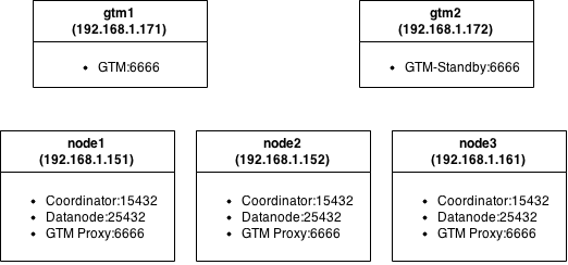
各ノードは、控えめなハードウェアを備えた仮想マシンです：MemTotal：501284 kB、cpu MHz：2604。

設置

ここではすべてが標準です：ソースをオフサイトからダウンロードし、依存関係を提供し、コンパイルします。 Ubuntuサーバー14.10。で収集されました。

$ sudo apt-get install flex bison docbook-dsssl jade iso8879 docbook libreadline-dev zlib1g-dev $ ./configure --prefix=/home/${USER}/Develop/utils/postgres-xl --disable-rpath $ make world
      
      

        
        
        
      

    
        
        
        
      
      

        
        
        
      

    
     

パッケージをアセンブルした後、クラスターのノードでパッケージを埋め、コンポーネントの構成に進みます。

GTMセットアップ

フォールトトレランスを確保するために、2つのGTMサーバーをセットアップする例を考えてください。 両方のサーバーで、GTMの作業ディレクトリを作成して初期化します。

 $ mkdir ~/gtm $ initgtm -Z gtm -D ~/gtm/
      
      

        
        
        
      

    
        
        
        
      
      

        
        
        
      

    
     

その後、構成設定に移動します。



gtm1



gtm2



保存して開始：

 $ gtm_ctl start -Z gtm -D ~/gtm/
      
      

        
        
        
      

    
        
        
        
      
      

        
        
        
      

    
     

ログでは、エントリを観察します：

ログ：GTM-Activeとして実行を開始しました。

ログ：GTM-St​​andbyとして実行を開始しました。

GTMプロキシの構成

 $ mkdir gtm_proxy $ initgtm -Z gtm_proxy -D ~/gtm_proxy/ $ nano gtm_proxy/gtm_proxy.conf
      
      

        
        
        
      

    
        
        
        
      
      

        
        
        
      

    
     

構成を編集した後、次を実行できます。

 $ gtm_ctl start -Z gtm_proxy -D ~/gtm_proxy/
      
      

        
        
        
      

    
        
        
        
      
      

        
        
        
      

    
     

コーディネーターを構成する

 $ mkdir coordinator $ initdb -D ~/coordinator/ -E UTF8 --locale=C -U postgres -W --nodename coordinator1 $ nano ~/coordinator/postgresql.conf
      
      

        
        
        
      

    
        
        
        
      
      

        
        
        
      

    
     

データノードのセットアップ

 $ mkdir ~/datanode $ initdb -D ~/datanode/ -E UTF8 --locale=C -U postgres -W --nodename datanode1 $ nano ~/datanode/postgresql.conf
      
      

        
        
        
      

    
        
        
        
      
      

        
        
        
      

    
     

他のノードの場合、設定は異なる名前を指定することによってのみ異なります。

pg_hba.confを編集します。

 echo "host all all 192.168.1.0/24 trust" >> ~/datanode/pg_hba.conf echo "host all all 192.168.1.0/24 trust" >> ~/coordinator/pg_hba.conf
      
      

        
        
        
      

    
        
        
        
      
      

        
        
        
      

    
     

起動とチューニング

すべて準備が整い、実行できます。

 $ pg_ctl start -Z datanode -D ~/datanode/ -l ~/datanode/datanode.log $ pg_ctl start -Z coordinator -D ~/coordinator/ -l ~/coordinator/coordinator.log
      
      

        
        
        
      

    
        
        
        
      
      

        
        
        
      

    
     

コーディネーターに行きます：

 psql -p15432
      
      

        
        
        
      

    
        
        
        
      
      

        
        
        
      

    
     

私たちは要求を満たします：

 select * from pgxc_node;
      
      

        
        
        
      

    
        
        
        
      
      

        
        
        
      

    
     

要求は、現在のサーバーがクラスターをどのように見るかを示します。

出力例：

  node_name | node_type | node_port | node_host | nodeis_primary | nodeis_preferred | node_id -------------+-----------+-----------+-----------+----------------+------------------+------------ coordinator1 | C | 5432 | localhost | f | f | 1938253334
      
      

        
        
        
      

    
        
        
        
      
      

        
        
        
      

    
     

これらの設定は間違っており、安全に削除できます。

 delete from pgxc_node;
      
      

        
        
        
      

    
        
        
        
      
      

        
        
        
      

    
     

クラスターの新しいマッピングを作成します。

 create node coordinator1 with (type=coordinator, host='192.168.1.151', port=15432); create node coordinator2 with (type=coordinator, host='192.168.1.152', port=15432); create node coordinator3 with (type=coordinator, host='192.168.1.161', port=15432); create node datanode1 with (type=datanode, host='192.168.1.151', primary=true, port=25432); create node datanode2 with (type=datanode, host='192.168.1.152', primary=false, port=25432); create node datanode3 with (type=datanode, host='192.168.1.161', primary=false, port=25432); SELECT pgxc_pool_reload(); select * from pgxc_node; node_name | node_type | node_port | node_host | nodeis_primary | nodeis_preferred | node_id --------------+-----------+-----------+---------------+----------------+------------------+------------- datanode1 | D | 25432 | 192.168.1.151 | t | f | 888802358 coordinator1 | C | 15432 | 192.168.1.151 | f | f | 1938253334 coordinator2 | C | 15432 | 192.168.1.152 | f | f | -2089598990 coordinator3 | C | 15432 | 192.168.1.161 | f | f | -1483147149 datanode2 | D | 25432 | 192.168.1.152 | f | f | -905831925 datanode3 | D | 25432 | 192.168.1.161 | f | f | -1894792127
      
      

        
        
        
      

    
        
        
        
      
      

        
        
        
      

    
     

残りのノードでも同じことをする必要があります。

データノードでは、情報を完全に消去することはできませんが、上書きすることはできます。

 psql -p 25432 -c "alter node datanode1 WITH ( TYPE=datanode, HOST ='192.168.1.151', PORT=25432, PRIMARY=true);"
      
      

        
        
        
      

    
        
        
        
      
      

        
        
        
      

    
     

クラスターテスト

これですべてが設定され、動作しました。 いくつかのテストテーブルを作成しましょう。

 CREATE TABLE test1 ( id bigint NOT NULL, profile bigint NOT NULL, status integer NOT NULL, switch_date timestamp without time zone NOT NULL, CONSTRAINT test1_id_pkey PRIMARY KEY (id) ) to node (datanode1, datanode2); CREATE TABLE test2 ( id bigint NOT NULL, profile bigint NOT NULL, status integer NOT NULL, switch_date timestamp without time zone NOT NULL, CONSTRAINT test2_id_pkey PRIMARY KEY (id) ) distribute by REPLICATION; CREATE TABLE test3 ( id bigint NOT NULL, profile bigint NOT NULL, status integer NOT NULL, switch_date timestamp without time zone NOT NULL, CONSTRAINT test3_id_pkey PRIMARY KEY (id) ) distribute by HASH(id); CREATE TABLE test4 ( id bigint NOT NULL, profile bigint NOT NULL, status integer NOT NULL, switch_date timestamp without time zone NOT NULL ) distribute by MODULO(status);
      
      

        
        
        
      

    
        
        
        
      
      

        
        
        
      

    
     

4つのテーブルが同じ構造で作成されましたが、クラスター全体で分散ロジックが異なります。



test1テーブルのデータは、 datanode1とdatanode2の 2つのデータノードにのみ格納され、ラウンドロビンアルゴリズムに従って分散されます。 残りのテーブルにはすべてのノードが含まれます。 test2テーブルはレプリケーションモードです。 test3テーブルのデータが保存されるサーバーを決定するには、 idフィールドにハッシュ関数を使用し、 test4の配布ロジックを決定するには、 statusフィールドにモジュールを使用します。 今すぐ記入してみましょう。

 insert into test1 (id, profile, status, switch_date) select a, round(random()*10000), round(random()*4), now() - '1 year'::interval * round(random() * 40) from generate_series(1,10) a; insert into test2 (id , profile,status, switch_date) select a, round(random()*10000), round(random()*4), now() - '1 year'::interval * round(random() * 40) from generate_series(1,10) a; insert into test3 (id , profile,status, switch_date) select a, round(random()*10000), round(random()*4), now() - '1 year'::interval * round(random() * 40) from generate_series(1,10) a; insert into test4 (id , profile,status, switch_date) select a, round(random()*10000), round(random()*4), now() - '1 year'::interval * round(random() * 40) from generate_series(1,10) a;
      
      

        
        
        
      

    
        
        
        
      
      

        
        
        
      

    
     

次に、このデータをリクエストして、スケジューラーがどのように機能するかを確認

 explain analyze select count(*) from test1; QUERY PLAN ------------------------------------------------------------------------------------------------------------------------------------- Aggregate (cost=27.50..27.51 rows=1 width=0) (actual time=0.649..0.649 rows=1 loops=1) -> Remote Subquery Scan on all (datanode1,datanode2) (cost=0.00..24.00 rows=1400 width=0) (actual time=0.248..0.635 rows=2 loops=1) Total runtime: 3.177 ms explain analyze select count(*) from test2; QUERY PLAN ------------------------------------------------------------------------------------------------------------------------------------- Remote Subquery Scan on all (datanode2) (cost=27.50..27.51 rows=1 width=0) (actual time=0.711..0.711 rows=1 loops=1) Total runtime: 2.833 ms explain analyze select count(*) from test3; QUERY PLAN ------------------------------------------------------------------------------------------------------------------------------------- Aggregate (cost=27.50..27.51 rows=1 width=0) (actual time=1.453..1.453 rows=1 loops=1) -> Remote Subquery Scan on all (datanode1,datanode2,datanode3) (cost=0.00..24.00 rows=1400 width=0) (actual time=0.465..1.430 rows=3 loops=1) Total runtime: 3.014 ms
      
      

        
        
        
      

    
        
        
        
      
      

        
        
        
      

    
     

スケジューラは、リクエストに参加するノードの数を通知します。 table2はすべてのノードに複製されるため、1つのノードのみがスキャンされます。 ちなみに、彼がどのロジックを選択したかは不明です。 彼がコーディネーターと同じノードからデータを要求することは論理的です。



データノード（ポート25432）に接続することにより、データがどのように分散されたかを確認できます。



次に、テーブルに大量のデータを入力し、クエリのパフォーマンスをスタンドアロンのPostgreSQLと比較してみましょう。

 insert into test3 (id , profile,status, switch_date) select a, round(random()*10000), round(random()*4), now() - '1 year'::interval * round(random() * 40) from generate_series(1,1000000) a;
      
      

        
        
        
      

    
        
        
        
      
      

        
        
        
      

    
     

Postgres-XLクラスターでのリクエスト：

 explain analyze select profile, count(status) from test3 where status<>2 and switch_date between '1970-01-01' and '2015-01-01' group by profile; QUERY PLAN --------------------------------------------------------------------------------------------------------------------------------------- HashAggregate (cost=34.53..34.54 rows=1 width=12) (actual time=266.319..268.246 rows=10001 loops=1) -> Remote Subquery Scan on all (datanode1,datanode2,datanode3) (cost=0.00..34.50 rows=7 width=12) (actual time=172.894..217.644 rows=30003 loops=1) Total runtime: 276.690 ms
      
      

        
        
        
      

    
        
        
        
      
      

        
        
        
      

    
     

PostgreSQLを使用するサーバーでの同じクエリ：

 explain analyze select profile, count(status) from test where status<>2 and switch_date between '1970-01-01' and '2015-01-01' group by profile; QUERY PLAN --------------------------------------------------------------------------------------------------------------------------------------- HashAggregate (cost=28556.44..28630.53 rows=7409 width=12) (actual time=598.448..600.495 rows=10001 loops=1) -> Seq Scan on test (cost=0.00..24853.00 rows=740688 width=12) (actual time=0.418..329.145 rows=740579 loops=1) Filter: ((status <> 2) AND (switch_date >= '1970-01-01 00:00:00'::timestamp without time zone) AND (switch_date <= '2015-01-01 00:00:00'::timestamp without time zone)) Rows Removed by Filter: 259421 Total runtime: 601.572 ms
      
      

        
        
        
      

    
        
        
        
      
      

        
        
        
      

    
     

速度が2倍になります。 それほど悪くはありませんが、十分な数の車を自由に使用できる場合、そのようなスケーリングは非常に有望に見えます。



コメントで述べたように、いくつかのノードに分散された結合テーブルを見るのは興味深いでしょう。 試してみましょう：

 create table test3_1 (id bigint NOT NULL, name text, CONSTRAINT test3_1_id_pkey PRIMARY KEY (id)) distribute by HASH(id); insert into test3_1 (id , name) select a, md5(random()::text) from generate_series(1,10000) a; explain analyze select test3.*,test3_1.name from test3 join test3_1 on test3.profile=test3_1.id; QUERY PLAN --------------------------------------------------------------------------------------------------------------------------------------- Remote Subquery Scan on all (datanode1,datanode2,datanode3) (cost=35.88..79.12 rows=1400 width=61) (actual time=26.500..17491.685 rows=999948 loops=1) Total runtime: 17830.984 ms
      
      

        
        
        
      

    
        
        
        
      
      

        
        
        
      

    
     

同じ量のデータを要求しますが、スタンドアロンサーバーで要求します。

  QUERY PLAN --------------------------------------------------------------------------------------------------------------------------------------- Hash Join (cost=319.00..42670.00 rows=999800 width=69) (actual time=99.697..19806.038 rows=999940 loops=1) Hash Cond: (test.profile = test_1.id) -> Seq Scan on test (cost=0.00..17353.00 rows=1000000 width=28) (actual time=0.031..6417.221 rows=1000000 loops=1) -> Hash (cost=194.00..194.00 rows=10000 width=41) (actual time=99.631..99.631 rows=10000 loops=1) Buckets: 1024 Batches: 1 Memory Usage: 713kB -> Seq Scan on test_1 (cost=0.00..194.00 rows=10000 width=41) (actual time=0.011..46.190 rows=10000 loops=1) Total runtime: 25834.613 ms
      
      

        
        
        
      

    
        
        
        
      
      

        
        
        
      

    
     

ここでは、ゲインはわずか1.5倍です。



PSこの投稿が誰かの役に立つことを願っています。 コメントや追加は大歓迎です！ ご清聴ありがとうございました。