
According to the Nilson report on the situation with bank cards and mobile payments, the total loss as a result of fraud in 2016 reached $ 22.8 billion, which is 4.4% more than in 2015. This only confirms the need for banks to learn to recognize fraud in advance, even before it takes place.
This is an extensive and very difficult task. Today, many methods have been developed, for the most part based on the direction of Data science, such as the detection of anomalies. Thus, depending on the available dataset, most of these techniques can be reduced to two main scenarios:
- Scenario 1: the dataset contains enough fraud patterns.
- Scenario 2: there are no (or negligible) fraud patterns in the dataset.
In the first case, we can solve the problem of fraud detection using classic machine learning techniques or statistical analysis. You can train the model or calculate the probabilities for two classes (legitimate and fraudulent transactions), and apply the model to new transactions to determine their legitimacy. In this case, all machine learning algorithms work with the teacher, designed to solve classification problems - for example, random forest, logistic regression, etc.
In the second case, we have no examples of fraudulent transactions, so we need to be creative. Since we only have samples of legitimate transactions, we need to make sure that this is enough. There are two options: consider fraud either as a deviation or as an anomalous value, and use the appropriate approach. In the first case, you can use an insulating forest , and in the second case, the classic solution is the auto-encoder .
Let's look at an example of a real dataset how to use different techniques. We implement them on a fraud detection dataset created by Kaggle. It contains 284,807 transactions with bank cards executed by Europeans in September 2013. For each transaction is presented:
- 28 main components extracted from the source data.
- How much time has passed since the first transaction in the dataset.
- Amount of money.
Transactions have two labels: 1 for fraudulent and 0 for legitimate (normal) ones. Only 492 (0.2%) transactions in the dataset are fraudulent, this is not enough, but it may be enough for some kind of training with a teacher.
Please note that for the sake of privacy, the data contains the main components instead of the original signs of transactions.
Scenario 1: Machine Learning with a Teacher - Random Forest
Let's start with the first scenario: suppose that we have a labeled dataset for teaching the classifying machine learning algorithm with a teacher. We can follow the classical design of a data analysis project: preparing information, training a model, evaluating and optimizing, deploying.
Information Preparation
This usually includes:
- Recover missing values if necessary for our algorithm.
- Choice of attributes to improve overall accuracy.
- Additional data transformations for compliance with privacy requirements.
In our case, the dataset is already cleaned and ready for use, no preparations are needed.
For all classifying algorithms with a teacher, training and test datasets are required. We can divide our array of information into two such datasets. Typically, their proportions range from 80% - 20% to 60% - 40%. We will divide in the ratio of 70% and 30%: most of the initial data will be used for training, and the remainder will be used to verify the operation of the resulting model.
To solve the classification problem that we are facing, we need to make sure that both datasets have samples of both classes - fraudulent and legitimate transactions. Since one class is much less common than the second, it is recommended to use stratified selection instead of random. Given the large imbalance between the two classes, stratified selection ensures that samples of all classes will be presented in both datasets according to their initial distribution.
Model training
We can use any algorithm with a teacher. Take a random forest with 100 trees. Each tree is trained to a depth of 10 levels, has no more than three samples per node. The algorithm uses information gain ratio to evaluate split criterion.
Model assessment: informed decision making
After training the model, you need to evaluate its performance on a test dataset. You can use classic assessment metrics , such as sensitivity and specificity, or the kappa coefficient (Cohen's Kappa). All measurements are based on forecasts made by the model. In most data analysis tools, models generate forecasts based on classes with the highest probability. In the binary classification problem, this is equivalent to using the default threshold of 0.5 for the probabilities of one of the classes.
However, when detecting fraudulent transactions, we may need a more conservative solution. It’s better to double-check legitimate transactions and risk worrying customers with a potentially useless call than skipping a fraudulent transaction. Therefore, we lower the threshold of acceptability for a fraudulent class, or increase this threshold for a legitimate one. In this case, we decided to take the threshold 0.3 for the probability of a fraudulent class and compare the results with the default threshold of 0.5.
Figure 1 shows the confusion matrix obtained at thresholds of 0.5 (left) and 0.3 (right). They correspond to the kappa coefficients 0.89 and 0.898 obtained on a sub-sampled dataset with the same number of legitimate and fraudulent transactions. As you can see, lowering the threshold for fraudulent transactions led to a false classification of several legitimate transactions, however, we correctly identified more fraudulent transactions.
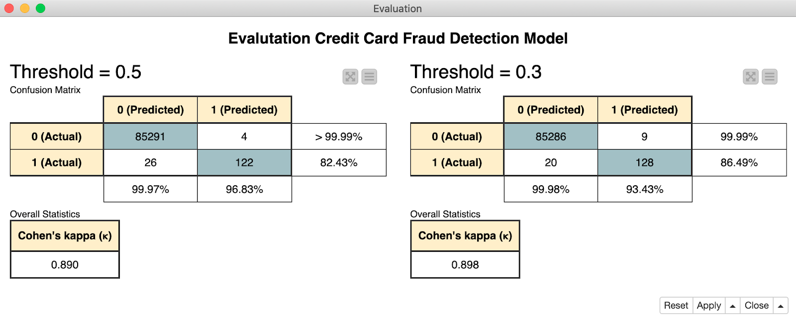
Figure 1. In the error matrices, class 0 corresponds to legitimate transactions, 1 to fraudulent transactions. By lowering the threshold to 0.3, we correctly identified 6 more fraudulent transactions.
Hyperparametric optimization
As in all classification decisions, to complete the training cycle, you can optimize the model parameters. For a random forest, this means finding the optimal number of trees and their depths to get the optimal classification quality (D. Goldmann, " Stuck in the Nine Circles of Hell? Try Parameter Optimization and a Cup of Tea "; KNIME Blog, 2018, Hyperparameter optimization ) . You can also optimize the prediction threshold.
We used a very simple learning process with only a few nodes (Figure 2): reading, dividing into training and test sets, training a random forest, generating a forecast, applying a threshold and assessing quality. We launched the " Fraud Detection: Model Training " process on the open source KNIME Analytics Platform.

Figure 2. This process reads the dataset and divides it into training and test sets. Then he trains a random forest, applies the resulting model to a test set and evaluates the quality of its work at thresholds of 0.3 and 0.5.
Deployment
When the quality of the model becomes satisfactory, you can use it to work with real data.
The deployment process (Figure 3) imports the trained model, reads one new transaction at a time, and applies the model and the selected threshold to it to get the final forecast. If the transaction is considered fraudulent, a letter is sent to the bank card holder to confirm the legitimacy of the transaction.
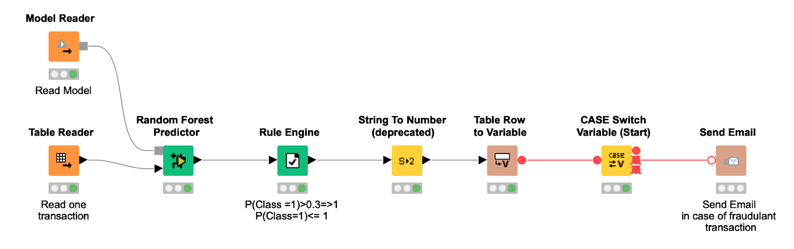
Figure 3. The deployment process reads the trained model and sends it one new transaction, applies the predicted probability threshold and sends a letter to the cardholder if the transaction is considered fraudulent.
Scenario 2: Anomaly Detection Using Auto-Encoder
Since there were very few fraudulent transactions in the original dataset, we can completely remove them from the training phase and use them only for testing.
One of the proposed approaches is based on anomaly detection techniques. These techniques are often used to search for any acceptable and unacceptable events in the data, whether it is hardware malfunctions on the Internet of things, an arrhythmic heartbeat during an ECG or fraudulent transactions with bank cards. The difficulty in detecting anomalies lies in the absence of abnormal patterns for training.
A technique such as a neural auto-encoder is often used: it is a neural architecture that can be trained on only one class of events and used to warn of unexpected new events.
AutoCoding Neural Architecture
As shown in Figure 4, an auto-encoder is a forward propagation neural network trained by back propagating an error. The network contains input and output layers, each of which consists of nodes. Between them is one or more hidden layers, and in the middle is the smallest layer, consisting of nodes ( ) The idea is to teach the neural network to reproduce the input vector x as an output vector .
The auto-encoder is trained only on samples of one or two classes, in our case these are legitimate transactions. After deployment, the auto-encoder will play the input as a day off , and for fraudulent transactions (anomalies), the result will not be optimal. Difference between and can be estimated by measuring the distance:
The final decision whether the transaction is legitimate or fraudulent is based on a threshold to distance . Transaction is a candidate for fraud in accordance with the rule for determining anomalies:
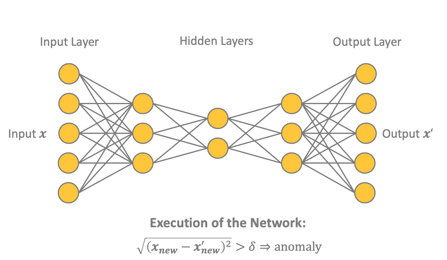
Figure 4. This shows a possible network structure of an auto-encoder. In this case, five input nodes and three hidden layers with three, two and three nodes, respectively. Output contains five nodes, like the input. To determine anomalies - fraudulent transactions - you can use the distance between the input and weekend .
Of course, you can set such a threshold value. so that the alarm works only in the most obvious cases of fraud. Or pick up depending on your needs and situation.
Let's look at the different stages of the process.
Data preparation
First, you need to make a subset of legitimate transactions into the training dataset. We used 90% of legitimate transactions for training an auto-encoder, and the remaining 10%, along with all fraudulent transactions, were placed in a test dataset.
Typically, data needs to be prepared in a training dataset. But it is already cleaned and ready for use. No further training is required. It is only necessary to perform this step: normalize the input vectors so that they fit into [0,1].
Creating and training an auto encoder
An autocoding network architecture is defined as 30-14-7-7-30. It uses tanh and ReLU activation functions, as well as an activity regularizer L1 = 0.0001, as suggested in the post " Credit Card Fraud Detection using Autoencoders in Keras - TensorFlow for Hackers (Part VII) ." Parameter L1 is a sparsity constraint, which reduces the likelihood of retraining a neural network.
The algorithm is trained until the final loss values fall within the range [0.070, 0.071] in accordance with the loss function in the form of a standard error:
Where - packet size, and - the number of nodes in the input and output layer.
Let’s set 50 epochs of training, we will also make the package size equal to 50. As a training algorithm, we take Adam , an optimized version of the inverse error distribution method . After training, save the neural network as a Keras file.
Model assessment: informed decision making
The value of the loss function does not give us the full picture. It only tells us how well the neural network can reproduce the “normal” input in the output layer. To get a complete picture of the quality of detection of fraudulent transactions, you need to apply the above mentioned anomaly detection rule to the test data.
To do this, determine the threshold to trigger a warning. You can start with the last value of the loss function at the end of the training phase. We used , but, as already mentioned, this parameter can be configured depending on your requirements for the conservatism of the neural network.
Figure 5 shows an assessment of the performance of a neural network in a test sample made using distance measurement.

Figure 5. Here is an assessment of the performance of the auto-encoder - error matrix and kappa coefficient. 0 denotes legitimate transactions, 1 - fraudulent.
The result was the following process: we collect a neural autocoder, divide the data into a training and test sample, normalize the data before feeding it into the neural network, train the neural network, run test data through it, calculate the distance apply the threshold value and evaluate the result. You can download the entire process here: Keras Autoencoder for Fraud Detection Training .

Figure 6. We read the dataset and break it into two samples: 90% of legitimate transactions in the training and the remaining 10% + all fraudulent transactions in the test. An auto-encoder neural network is defined in the upper left of the circuit. After normalizing the data, we train the auto-encoder and evaluate its work.
Deployment
Please note that the neural network itself and the threshold rule were deployed in a REST application, which receives input from a REST request and generates a forecast in a REST response.
The deployment process is shown below, download it here: Keras Autoencoder for Fraud Detection Deployment .

Figure 7. Execution of this process can be started from any application by sending a new transaction in a REST request. The process reads and applies the model to the input, and then sends a response with a forecast: 0 for a legitimate transaction or 1 for a fraudulent one.
Deviation Detection: Isolation Forest
In the absence of fraud patterns, another group of strategies can be applied based on deviation detection techniques. We chose an isolation forest (M. Widmann and M. Heine, “ Four Techniques for Outlier Detection ,” KNIME Blog, 2019).
The essence of the algorithm is that the deviation can be isolated using fewer random divisions as compared to the standard class, since deviations are less common and do not fit into the statistics of the dataset.
The algorithm randomly selects a characteristic, and then randomly selects a value from the range of this characteristic as a split value. By recursively applying this split procedure, a tree is generated. The depth of the tree is determined by the number of necessary random partitions (isolation level) for isolating the sample. The isolation level (often referred to as mean length) averaged over the forest of such random trees is a measure of normality and our decision function for detecting deviations. Random partitioning makes trees for deviations significantly shorter, and for normal samples - longer. Therefore, if a forest of random trees for a specific pattern generates shorter paths, then this is probably a deviation.
Data preparation
Data is prepared in the same way as described above: restoration of missing values, selection of features, additional data transformations to comply with the requirements of the privacy regulator. Since this dataset has already been cleared, you can use it; no additional preparation is required. Training and test samples are created in the same way as for the auto-encoder.
Training and use of the insulating forest
We trained a forest of 100 trees with a maximum depth of 8 and for each transaction we calculated the average isolation level for all trees in the forest.
Model assessment: informed decision making
Remember that the average isolation level for deviations is lower than for other data units. We have taken the threshold . Consequently, a transaction is considered fraudulent if the average isolation level is below this value. As in the two previous examples, the threshold value can be selected depending on the desired model sensitivity.
The effectiveness of this approach in the test sample is shown in Figure 8. The final process, which can be downloaded from here , is shown in Figure 9.

Figure 8. Evaluation of the effectiveness of an insulating forest on the same test set that was used for the auto-encoder.
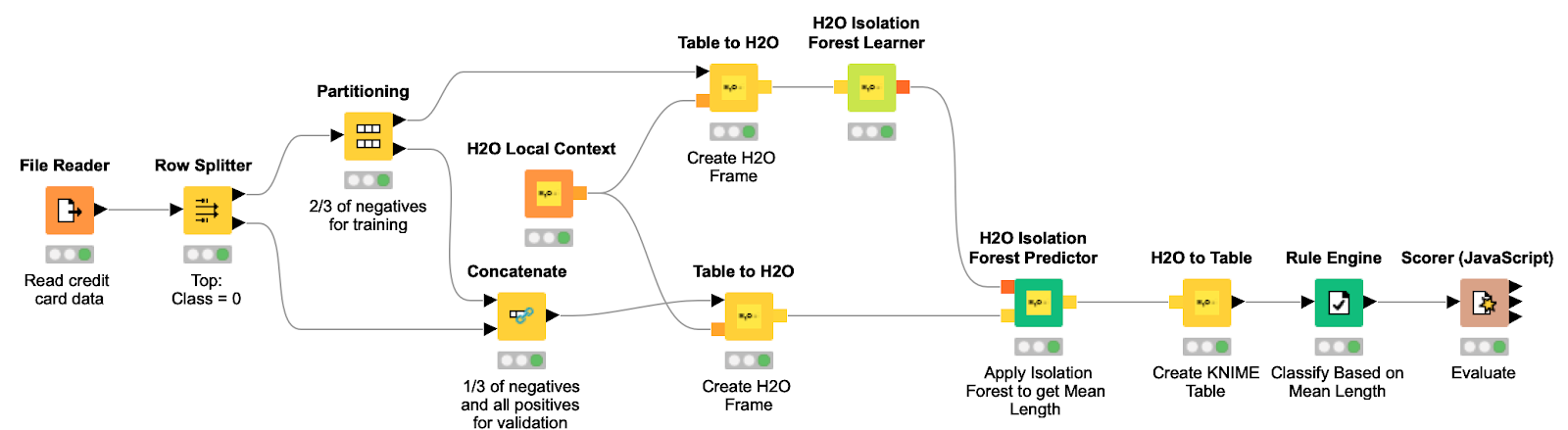
Figure 9. This process reads the dataset, creates a training and test sample, and converts them to H2O Frame. He then trains the isolation forest and applies the model to the test suite to find variances using the isolation level for each transaction.
Deployment
The process reads the isolation forest model and applies it to the new input. Based on the threshold defined during training and applied to the isolation level, the model identifies incoming transactions as legitimate or fraudulent.
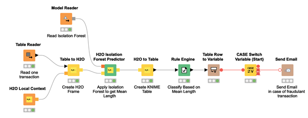
Figure 10. A process reads a new transaction and applies a trained isolation forest model to it. For each input transaction, the isolation level is calculated and a decision is made whether the transaction is fraudulent. If so, a letter is sent to the bank card holder.
Summary
Fraud detection is an extensive area of research in the field of data analysis. We described two possible scenarios depending on the available dataset: either with samples of legitimate and fraudulent transactions, or completely fraudulent (with a negligible amount).
In the first case, we proposed a classical approach based on a machine learning algorithm with a teacher, with all the steps taken in the data analysis projects described in the CRISP-DM process. This is the recommended approach. In particular, we implemented a classifier based on a random forest.
In some situations, it is necessary to solve the problem of detecting fraud without having samples in hand. In such cases, less accurate approaches can be used. We have described yes from them: an auto-encoder neural network from anomaly detection methods and an isolating forest from deviation detection methods. They are not as accurate as a random forest, but in some cases there are simply no alternatives.
Of course, these are not the only possible approaches, but they represent three popular groups of solutions for the task of detecting fraud.
Please note that the last two approaches were used in situations where there is no access to marked up fraudulent transactions. These are some kind of forced approaches that can be used if it is impossible to use the classical classification solution. If possible, use a classifier algorithm with the teacher. But if there is no information about fraud, the last two approaches described will help. They give false positives, but sometimes there are simply no other ways.