“You'll know it from a thousand ...” or classify images from a webcam in real time using PyTorch

Here it happens in life. You’re sitting around being naughty, don’t bother anyone, fixing up the stove, and here from this stove, from the TV, and indeed from every iron, you hear: “neural networks, deep learning, artificial intelligence, digital economy ...”.



I am a man, which means a curious and greedy creature. Once again, I could not resist and decided to find out in practice what neural networks are and what they eat with.

As the saying goes: "If you want to learn yourself, start teaching others," on this I will stop pouring quotes and get down to business.



In this article, we will try to solve a problem with you, which, as it turned out, excites not only my mind.

Without sufficient fundamental knowledge in the field of mathematics and programming, we will try in real time to classify images from a webcam using OpenCV and the Python machine learning library PyTorch. Along the way, we learn about some points that could be useful to beginners in the use of neural networks.



Are you curious if our classifier can distinguish Arduino-compatible controllers from raspberries? Then you are welcome under cat.







Content:



Part I: Introduction

Part II: image recognition using neural networks

Part III: getting ready to use PyTorch

Part IV: Writing Python Code

Part V: the fruits of labor

Part I: Introduction

To be honest, almost immediately after completing the specialization in Machine Learning Coursera , I wanted to prepare some material in a series of articles on machine learning through the eyes of a beginner.





However, to gather strength and write it turned out only now.



First you need to warn, think well, are you ready to immerse yourself in this wonderful world?



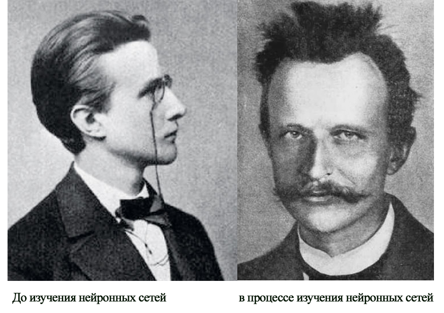
It took me four full days off and a couple of weekly evenings to prepare this article. And also a bunch of unsuccessful attempts to deal with the issue without prior preparation. Therefore, in this case, it will be appropriate to re-edit the well-known graphic humoresque with Max Planck.







It must also be said that to understand the code examples from this article, basic knowledge of the Python language and its common libraries used for machine learning (for example, NumPy) will still be necessary.



This article will not have theoretical calculations or a detailed description of neural networks and the principles of their work, since it is not decent to try to talk smartly about what he did not fully understand. Therefore, we just see how I was tormented, try not to make the same mistakes, and in the end we can even recognize something.



Are you still reading this text? Great, now I am confident in the strength of your spirit and stamina.

Part II: image recognition using neural networks

Thanks to the fact that a lot of smart and probably talented people are involved in the development of everything related to neural networks, there are many free tools and examples for solving problems from recognizing car numbers to translating texts.



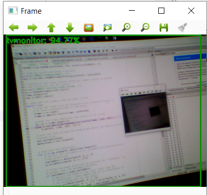
You want to use a webcam with high reliability to recognize that you have a person or a monitor, it’s not a question, we just find an implemented example , copy less than a hundred lines of code and voila “voila ” .











All this can create a deceptive illusion of simplicity.

Difficulties arise if you want to do something of your own. After all, you always want to, if you don’t already assemble your bike, then at least fasten a cool horn and a flashlight to it.



So, in the example above, we meet a function:

net = cv2.dnn.readNetFromCaffe(args_prototxt, args_model)
      
      

        
        
        
      

    
        
        
        
      
      

        
        
        
      

    
     

Which clearly hints, even to an untrained person, that something called “Caffe” is used for the neural network.



As it turned out, Caffe is a deep machine learning framework.



It is difficult to say that I didn’t like out of ignorance, maybe the project site with boring wallpapers , maybe TensorFlow was just a rumor, but I firmly decided that I would not start with Caffe.



Do not think anything, I do not want to criticize Caffe, I assume that this is a good framework, just the first impression did not work out. I will surely return to him, sometime later .



Well then, take a look at TensorFlow. If you believe the Russian-language Wikipedia:

TensorFlow is an open software library for machine learning developed by Google to solve the problems of building and training a neural network in order to automatically find and classify images, achieving the quality of human perception.

I decided that it was very cool, I ran to poke into all the tutorials that came across, including the training of ready-made models for classifying images on my data sets .



After short moments of glee, I joyfully find the OpenCV method:

 cv.dnn.readNetFromTensorflow(model[, config] )
      
      

        
        
        
      

    
        
        
        
      
      

        
        
        
      

    
     

And then joyfully run to the Internet to replenish the line of people asking the following questions:

"How to convert a model in .h5 to .pb file"

“How to get a frozen _ .pb file”

“How to make a .pbtxt from a .pb file”

For a long time I did not feel such unity as with people asking these and other amateurish questions on Stack overflow.



Moreover, in all the examples that I came across there was some kind of catch and something didn’t work even the OpenCV example gave an error at startup.



As a result, the first week was spent on trying, without delving into the details and not studying the basics, to achieve at least something from TensorFlow and OpenCV.



But after one of the days at four o’clock in the morning, the program looked at me with its impartial eye of the webcam and said that I was 22% likely to be an airplane , I realized that it was time to change something in the approach to case.



As with Caffe, I ask you not to think that I have something against TensorFlow. This is a very cool library with a huge community, I just could not take it by storm, I was disappointed and went to look for a solution further. But in fact, I will definitely come back to her more prepared and write a short article about it.



In the meantime, we continue to track the throwing of an excited and saddened by failure of mind.

Let's look again at what OpenCV methods are for working with neural networks and find:

 cv.dnn.readNetFromTorch(model[, isBinary[, evaluate]])
      
      

        
        
        
      

    
        
        
        
      
      

        
        
        
      

    
     

Wow! Looks like it's time to get acquainted with another machine learning library.

Part III: Getting Ready to Use PyTorch

As PyTorch said , this is another fairly popular machine learning framework that people from Facebook had a hand in. Subjectively, it seemed to me that the PyTorch website has fewer training examples and that the framework’s community is somewhat smaller than TensorFlow’s, but looking ahead I’ll say what exactly I managed to do with it, almost what was originally intended.



So, as I wrote above in the second week, it came to the understanding that simply copying other people's examples into the blind without understanding what you are doing in the hope of building a ready-made model and recognizing an image from a webcam using OpenCV is a way to nowhere.



Therefore, it was decided to write a script in parallel and learn about neural networks.

A very good help in this matter is the book of Rashid Tarik “We create a neural network”, it was already mentioned on Habré habr.com/en/post/440190 . This book is written in very accessible language about the basic concepts of neural networks, but, of course, it will not teach us how to use PyTorch.



Therefore, it will not be superfluous to run a tutorial about deep learning with PyTorch in 60 minutes . It really will not take much time, but it will give at least a partial understanding of the basic principles of work. You can execute code both on Google Colab and locally.



So we smoothly approached the question of how to write code on our machine.



On the official website, we will be offered various installation options depending on the operating system, the desired version of python and the installation method.



For beginners who love Python machine learning, I suggest installing PyTorch using the Anaconda distribution , which works well on both Windows and Linux.



Then create a separate environment in Anaconda for our experiments and begin to slowly install all the necessary packages there, including OpenCV.



You can install PyTorch in Anaconda either through the graphical interface or through the console (Anaconda Prompt for Windows).











For image recognition we need a tourchvision library.



It is also possible in the text entered into the console you already saw “cudatoolkit = 10.1” and you had a question what CUDA is, which version should be installed and whether it should be installed at all.



As I understand it, CUDA allows you to transfer calculations from the processor to the video card from Nvidia. Judging by the reviews, this speeds up the process of calculating the model at times. But there is a fly in the ointment in the ointment, if you, like me, are a lucky owner of an ancient video card, then after installation, when you try to use CUDA PyTorch, you may be asked to update the video driver first, and then break all the hopes, saying that your video card is too old and not supported.



For example, my GTX 760 seems to be supported by CUDA version 3.5. I did not find the list of video cards supported by this or that version of CUDA, but I think that all owners of fairly old video cards may not hesitate between version 9.2 and 10.1, but immediately install the version without its support.



There are literally the final touches before we start writing code.



We want the model to recognize objects close to our heart, which means we need to assemble our own set of images.



In this case, the torchvision.datasets.ImageFolder class will help us, which, in conjunction with the torch.utils.data.DataLoader class, allows you to create your own dataset from a structured set of image folders.



The structure of our image set will look something like this:











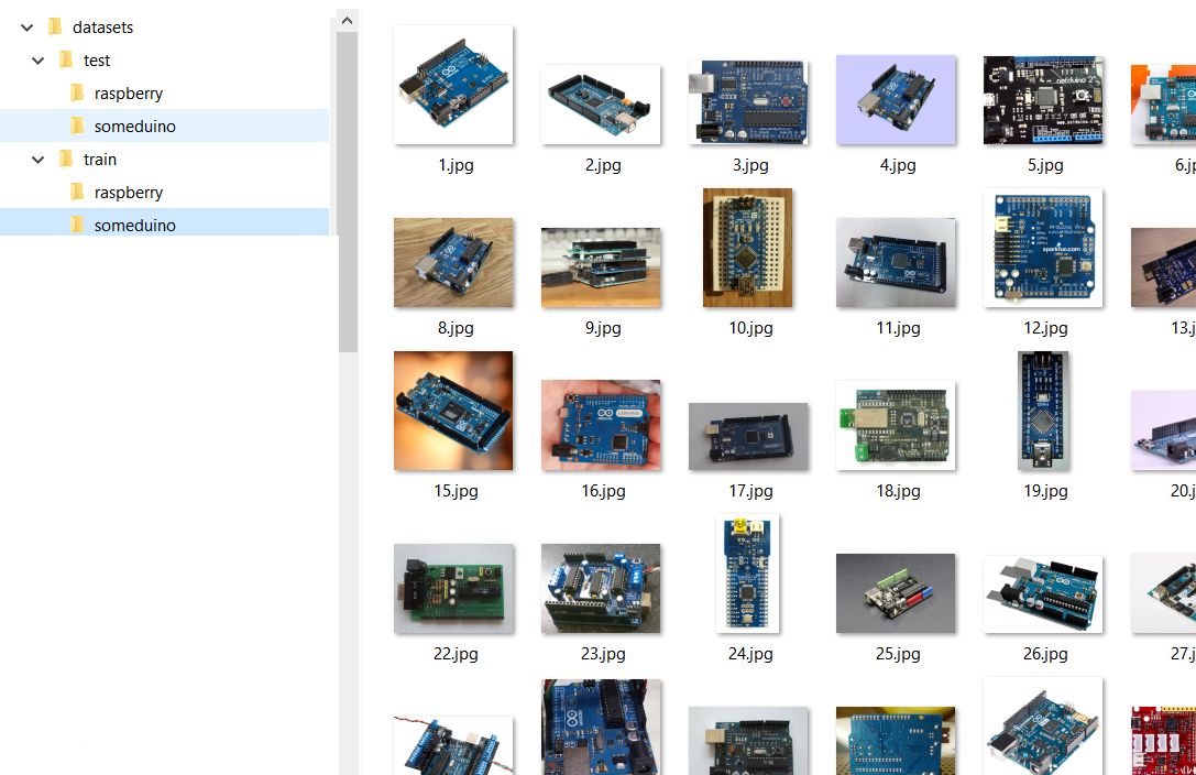
That is, we have the Test and Train folders in which the folders with recognized classes of the classes “someduino” and “raspberry” are located. In the training sample, for each class, 128 images are presented in the test sample - 28. I must say that a good neural network must be learned from scratch on millions or at least hundreds of thousands of images, but we don’t set any practical tasks for ourselves and try to cope with the fact that managed to collect.



By the way, two words about collecting images for your dataset.



If you want to put the dataset on the network and not have nightmares about copyright infringement, I recommend using images of rights to that allow you to do this.



You can find them, for example, using the search on Google images, by selecting the appropriate item in the search filters, as shown in the figure below.











Well, part of the images can always be done independently.



I should apologize if I am embarrassed, maybe from the title picture of the article you thought that we would compare the images of Arduino and raspberry pi, however for the big differences between the classes, we will compare the images of different versions of Arduino (and its clones) with raspberry.

Part IV: Writing Python Code

So we got to the most interesting.

As always, all the materials in this article, including images, I posted on GitHub for free access.



We start with a Jupyter notebook in which we will train the model.



The notebook is divided into two logical parts, one is dedicated to creating a simple model and learning it from scratch, and in the other we will apply transfer learning to a ready-made and trained model.

In the first case, we focus on this tutorial .



I practically didn’t rule anything in the materials from the tutorial, because I was afraid to break something that I don’t understand well, so basically you can study the above example and achieve similar results.



To get started, we import the necessary libraries (make sure that you have installed them).

 from __future__ import print_function, division import torch import torch.nn as nn import torch.optim as optim from torch.optim import lr_scheduler import numpy as np import matplotlib.pyplot as plt import torchvision from torchvision import datasets, models import torchvision.transforms as transforms import matplotlib.pyplot as plt import time import os import copy import torch.nn as nn import torch.nn.functional as F import torch.optim as optim from torch.autograd import Variable import torch.onnx import torchvision %matplotlib inline plt.ion() # interactive moden
      
      

        
        
        
      

    
        
        
        
      
      

        
        
        
      

    
     

Then we will determine the address from which we will load the dataset

 #get address such as C:\\(folder with you notebook) dir = os.path.abspath(os.curdir) # i suppose what your image folders placed in datasets directory data_dir=os.path.join(dir, "datasets\\")
      
      

        
        
        
      

    
        
        
        
      
      

        
        
        
      

    
     

Below is the code for transforming the image, in which, if necessary, we reduce, crop, darken or brighter the data before feeding their models.



In our case, we reduce the image to 32x32 pixels and normalize it (we won’t go into math now).

 # Data scaled and normalization for training and testing data_transforms = { 'train': transforms.Compose([ transforms.RandomResizedCrop(32), transforms.ToTensor(), transforms.Normalize([0.5, 0.5, 0.5], [0.5, 0.5, 0.5]) ]), 'test': transforms.Compose([ transforms.RandomResizedCrop(32), transforms.ToTensor(), transforms.Normalize([0.5, 0.5, 0.5], [0.5, 0.5, 0.5]) ]), }
      
      

        
        
        
      

    
        
        
        
      
      

        
        
        
      

    
     

Next, we will write a function that converts our images into an array of data (tensors) for further training. The function is slightly different from the one presented in the example, since we will use it twice, not only the path to the folder, but also the conversion scheme is used as input parameters.

 #Create function to get your(my) images dataset and resize it to size for model def get_dataset(data_dir, data_transforms ): # create train and test datasets image_datasets = {x: datasets.ImageFolder(os.path.join(data_dir, x), data_transforms[x]) for x in ['train', 'test']} dataloaders = {x: torch.utils.data.DataLoader(image_datasets[x], batch_size=4, shuffle=True, num_workers=4) for x in ['train', 'test']} dataset_sizes = {x: len(image_datasets[x]) for x in ['train', 'test']} #get classes from train dataset folders name classes = image_datasets['train'].classes return dataloaders["train"], dataloaders['test'], classes, dataset_sizes
      
      

        
        
        
      

    
        
        
        
      
      

        
        
        
      

    
     

At the output, the function returns two datasets in the format necessary for our neural network model, and as a bonus, information about image classes obtained from the name of the folders, and the size of the training and training samples.



When you make your dataset, make sure that the folder structures of train and test are identical (the same number of classes), and also that you used .jpg images. Sometimes, under the guise of an innocent picture, any garbage creeps in, which causes an error during processing.



We use the newly created function.

 trainloader, testloader, classes, dataset_sizes=get_dataset(data_dir,data_transforms) print('Classes: ', classes) print('The datasest have: ', dataset_sizes ," images")
      
      

        
        
        
      

    
        
        
        
      
      

        
        
        
      

    
     

As expected, we have only two classes: the proletariat and the bourgeoisie 'raspberry' and 'someduino'.



The training sample contains 256 images, the control 56.



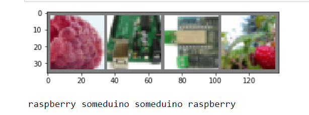
Let's see how our data looks in the training set.

 # create function for print unnormalized images def imshow(img): img = img / 2+0.5 # unnormalize npimg = img.numpy() plt.imshow(np.transpose(npimg, (1, 2, 0))) plt.show() # get some random training images dataiter = iter(trainloader) images, labels = next(dataiter) #images, labels = dataiter.next() # show images imshow(torchvision.utils.make_grid(images)) # print labels print(' '.join('%5s' % classes[labels[j]] for j in range(4)))
      
      

        
        
        
      

    
        
        
        
      
      

        
        
        
      

    
     

If by eye we can distinguish between objects in a 32x32 image, then our neural network should be able to.











Further, the model itself.



Here we create layers with different dimensions of input and output, as well as functions due to which transformations will be carried out. Unfortunately, this stage in my head did not completely fit in, so we just use it, the main thing is that it works.

 class Net(nn.Module): def __init__(self): super(Net, self).__init__() self.conv1 = nn.Conv2d(3, 6, 5) self.pool = nn.MaxPool2d(2, 2) self.conv2 = nn.Conv2d(6, 16, 5) self.fc1 = nn.Linear(16 * 5 * 5, 120) self.fc2 = nn.Linear(120, 84) self.fc3 = nn.Linear(84, 2) def forward(self, x): x = self.pool(F.relu(self.conv1(x))) x = self.pool(F.relu(self.conv2(x))) x = x.view(-1, 16 * 5 * 5) x = F.relu(self.fc1(x)) x = F.relu(self.fc2(x)) x = self.fc3(x) return x net = Net() print(net)
      
      

        
        
        
      

    
        
        
        
      
      

        
        
        
      

    
     

At the end of this piece of code, we actually created our neural network.



If you want more classes, then try replacing a two with a three in the line below.

  self.fc3 = nn.Linear(84, 2)
      
      

        
        
        
      

    
        
        
        
      
      

        
        
        
      

    
     

It remains to teach the model something.

 criterion = nn.CrossEntropyLoss() optimizer = optim.SGD(net.parameters(), lr=0.001, momentum=0.9) device = torch.device("cpu") for epoch in range(11): # loop over the dataset multiple times running_loss = 0.0 for i, data in enumerate(trainloader, 0): # get the inputs; data is a list of [inputs, labels] inputs, labels = data # zero the parameter gradients optimizer.zero_grad() # forward + backward + optimize outputs = net(inputs) loss = criterion(outputs, labels) loss.backward() optimizer.step() # print statistics running_loss += loss.item() if i % 15 == 14: # print every 15 mini-batches print('[%d, %5d] loss: %.3f' % (epoch + 1, i + 1, running_loss / 15)) running_loss = 0.0 print('Finished Training')
      
      

        
        
        
      

    
        
        
        
      
      

        
        
        
      

    
     

In the above code snippet, we first defined the optimization and completion criteria. And then they began to teach our model for 11 eras.



The more eras, the better the model should learn (less prediction error), but the more time is required. Our model (most likely), due to random mixing of datasets, will produce a different error each time, but by the 11th era it will still tend closer to zero.



In this cycle, for clarity, information on the progress of training is periodically displayed.

This is what the model produces on my computer. The text is long shoved to hide under the spoiler.





It's time to check on a control sample whether our model is able to classify pictures.

 correct = 0 total = 0 with torch.no_grad(): for data in testloader: images, labels = data outputs = net(images) _, predicted = torch.max(outputs.data, 1) for printdata in list(zip(predicted,labels,outputs)): printclass =[classes[int(printdata[0])],classes[int(printdata[1])]] print('Predict class - {0}, real class - {1}, probability ({2},{3}) - {4}'.format( printclass[0],printclass[1], classes[0], classes [1],printdata[2])) total += labels.size(0) correct += (predicted == labels).sum().item() imshow(torchvision.utils.make_grid(images)) #print('GroundTruth: ', ' '.join('%5s' % classes[predicted[j]] for j in range(4))) print('Accuracy of the network on the', dataset_sizes['test'], 'test images: %d %%' % ( 100 * correct / total))
      
      

        
        
        
      

    
        
        
        
      
      

        
        
        
      

    
     

We run the code and see that yes it is quite capable. But if we spent only 2 - 3 eras, the result would be disastrous.











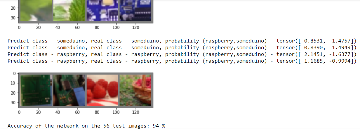
Naturally, you will be shown the results for all 28 control images, just for obvious reasons, they did not fit into the picture.



Next comes an optional code. It shows how to save and load the model, and also re-displays the analysis of control images, confirming that the quality has not deteriorated.

 #(Optional) #Save and load model PATH =os.path.join(dir, "my_model.pth") torch.save(net.state_dict(), PATH) net = Net() net.load_state_dict(torch.load(PATH))
      
      

        
        
        
      

    
        
        
        
      
      

        
        
        
      

    
     

The code with the output of the images is similar to the one above.



Well, that’s all we trained our first model to recognize images, it remains the case for small insert its saved version into the function

 cv.dnn.readNetFromTorch("my_model.pth")
      
      

        
        
        
      

    
        
        
        
      
      

        
        
        
      

    
     

But oh, horror! This code will throw an error, because the PyTorch dictionary and the model file that Tourch saves are not the same thing, but the Torch model is expected from us here.











Do not panic. Once again, we look at what models OpenCV can work with and find

 cv.dnn.readTensorFromONNX(path)
      
      

        
        
        
      

    
        
        
        
      
      

        
        
        
      

    
     

Here it is our wonderful compromise. It remains only to convert our model to .onnx

 # Export model to onnx format PATH =os.path.join(dir, "my_model.onnx") #(1, 3, 32, 32) –   , 3   3232 , dummy_input = Variable(torch.randn(1, 3, 32, 32)) torch.onnx.export(net, dummy_input, PATH)
      
      

        
        
        
      

    
        
        
        
      
      

        
        
        
      

    
     

Looking ahead, I’ll say that everything will work great, but before moving on to working with a webcam. Let's try to take a better model and train it on our data set.



This half of the notebook will be based on this tutorial and we will train the resnet18 model



Pay attention to this model, a slightly different preparation of the source data is needed. As a rule, you can read about the conversion parameters in the descriptions of the model or simply borrowing someone else's example.

 #Data scaled and normalization for training and testing for resnet18 data_transforms = { 'train': transforms.Compose([ transforms.RandomResizedCrop(224), transforms.RandomHorizontalFlip(), transforms.ToTensor(), transforms.Normalize([0.485, 0.456, 0.406], [0.229, 0.224, 0.225]) ]), 'test': transforms.Compose([ transforms.Resize(256), transforms.CenterCrop(224), transforms.ToTensor(), transforms.Normalize([0.485, 0.456, 0.406], [0.229, 0.224, 0.225]) ]), }
      
      

        
        
        
      

    
        
        
        
      
      

        
        
        
      

    
     

Next comes, in fact, a similar code, preparing datasets and viewing pictures, we will leave it without comment.

 # get train and test data trainloader, testloader, classes, dataset_sizes=get_dataset(data_dir, data_transforms) print('Classes: ', classes) print('The datasest have: ', dataset_sizes ," images") # Create new image show function for new transofration def imshow_resNet18(inp, title=None): """Imshow for Tensor.""" inp = inp.numpy().transpose((1, 2, 0)) mean = np.array([0.485, 0.456, 0.406]) std = np.array([0.229, 0.224, 0.225]) inp = std * inp + mean inp = np.clip(inp, 0, 1) plt.imshow(inp) if title is not None: plt.title(title) plt.pause(0.001) # pause a bit so that plots are updated # get some random training images dataiter = iter(trainloader) images, labels = next(dataiter) #images, labels = dataiter.next() # show images imshow_resNet18(torchvision.utils.make_grid(images)) # print labels print(' '.join('%5s' % classes[labels[j]] for j in range(4)))
      
      

        
        
        
      

    
        
        
        
      
      

        
        
        
      

    
     

And here is the function for training the model. I did not understand half of it, so for now just use it as it is.

 def train_model(model, criterion, optimizer, scheduler, num_epochs=25): since = time.time() best_model_wts = copy.deepcopy(model.state_dict()) best_acc = 0.0 for epoch in range(num_epochs): print('Epoch {}/{}'.format(epoch, num_epochs - 1)) print('-' * 10) # Each epoch has a training and validation phase for phase in ['train', 'test']: if phase == 'train': model.train() # Set model to training mode else: model.eval() # Set model to evaluate mode running_loss = 0.0 running_corrects = 0 # Iterate over data. for inputs, labels in dataloaders[phase]: inputs = inputs.to(device) labels = labels.to(device) # zero the parameter gradients optimizer.zero_grad() # forward # track history if only in train with torch.set_grad_enabled(phase == 'train'): outputs = model(inputs) _, preds = torch.max(outputs, 1) loss = criterion(outputs, labels) # backward + optimize only if in training phase if phase == 'train': loss.backward() optimizer.step() # statistics running_loss += loss.item() * inputs.size(0) running_corrects += torch.sum(preds == labels.data) if phase == 'train': scheduler.step() epoch_loss = running_loss / dataset_sizes[phase] epoch_acc = running_corrects.double() / dataset_sizes[phase] print('{} Loss: {:.4f} Acc: {:.4f}'.format( phase, epoch_loss, epoch_acc)) # deep copy the model if phase == 'test' and epoch_acc > best_acc: best_acc = epoch_acc best_model_wts = copy.deepcopy(model.state_dict()) print() time_elapsed = time.time() - since print('Training complete in {:.0f}m {:.0f}s'.format( time_elapsed // 60, time_elapsed % 60)) print('Best val Acc: {:4f}'.format(best_acc)) # load best model weights model.load_state_dict(best_model_wts) return model
      
      

        
        
        
      

    
        
        
        
      
      

        
        
        
      

    
     

In this code, it’s also difficult for me to comment on anything.

 # Let's prepare the parameters for training the model dataloaders = {'train': trainloader, 'test': testloader} model_ft = models.resnet18(pretrained=True) num_ftrs = model_ft.fc.in_features # Here the size of each output sample is set to 2. # Alternatively, it can be generalized to nn.Linear(num_ftrs, len(class_names)). model_ft.fc = nn.Linear(num_ftrs, 2) model_ft = model_ft.to(device) criterion = nn.CrossEntropyLoss() # Observe that all parameters are being optimized optimizer_ft = optim.SGD(model_ft.parameters(), lr=0.001, momentum=0.9) # Decay LR by a factor of 0.1 every 7 epochs exp_lr_scheduler = lr_scheduler.StepLR(optimizer_ft, step_size=7, gamma=0.1)
      
      

        
        
        
      

    
        
        
        
      
      

        
        
        
      

    
     

But still I will comment on something.

 dataloaders = {'train': trainloader, 'test': testloader}
      
      

        
        
        
      

    
        
        
        
      
      

        
        
        
      

    
     

This dictionary was necessary so as not to touch anything in the learning function of the model from the tutorial, but at the same time keep the previously written function for preparing the dataset.

And the second important point, as in the past case, if you want more classes, replace the two.

 model_ft.fc = nn.Linear(num_ftrs, 2)
      
      

        
        
        
      

    
        
        
        
      
      

        
        
        
      

    
     

I think it should work.



Train the model.

 #Train the model model_ft = train_model(model_ft, criterion, optimizer_ft, exp_lr_scheduler, num_epochs=5)
      
      

        
        
        
      

    
        
        
        
      
      

        
        
        
      

    
     

Pay attention to us, fewer eras to get an error no worse than the first model in 11 eras.











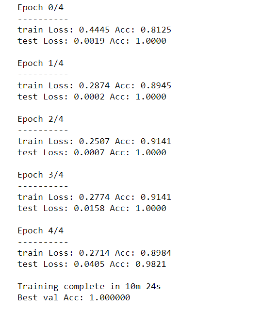
True, each era takes many times more time. For more complex tasks, of course, you will need more eras.



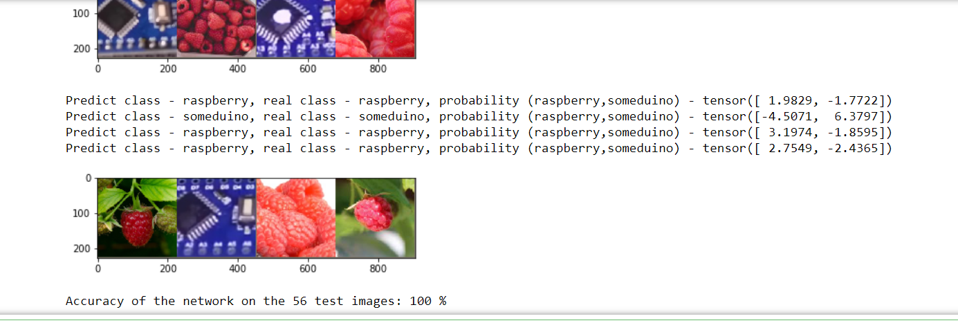
I replaced the verification of recognizable images from the original tutorial with a slightly adapted code that we used to visualize the recognition results of the test sample of the first model.

 # Visualization results of analysis test data correct = 0 total = 0 with torch.no_grad(): for data in testloader: images, labels = data outputs = model_ft(images) _, predicted = torch.max(outputs.data, 1) for printdata in list(zip(predicted,labels,outputs)): printclass =[classes[int(printdata[0])],classes[int(printdata[1])]] print('Predict class - {0}, real class - {1}, probability ({2},{3}) - {4}'.format( printclass[0],printclass[1], classes[0], classes [1],printdata[2])) total += labels.size(0) correct += (predicted == labels).sum().item() imshow_resNet18(torchvision.utils.make_grid(images)) #print('GroundTruth: ', ' '.join('%5s' % classes[predicted[j]] for j in range(4))) print('Accuracy of the network on the', dataset_sizes['test'], 'test images: %d %%' % ( 100 * correct / total))
      
      

        
        
        
      

    
        
        
        
      
      

        
        
        
      

    
     

Recognized - perfect.











It remains to save.

 # Export model to onnx format PATH =os.path.join(dir, "my_resnet18.onnx") dummy_input = Variable(torch.randn(1, 3, 224, 224)) torch.onnx.export(model_ft, dummy_input, PATH)
      
      

        
        
        
      

    
        
        
        
      
      

        
        
        
      

    
     

Part V: The fruits of labor

The only thing left is to “feed” the saved models in OpenCV.



I was guided by this example , but in principle you can easily write your own.



First, import the libraries.

 # import the necessary packages from imutils.video import VideoStream from imutils.video import FPS import numpy as np import imutils import time import cv2 import os
      
      

        
        
        
      

    
        
        
        
      
      

        
        
        
      

    
     

Then - the preparatory stage.

 path=os.path.join(os.path.abspath(os.curdir) , 'my_model.onnx') args_confidence = 0.2 # initialize the list of class labels CLASSES = ['raspberry', 'someduino'] # load our serialized model from disk print("[INFO] loading model...") net = cv2.dnn.readNetFromONNX (path) # initialize the video stream, allow the c #cammera sensor to warmup, # and initialize the FPS counter print("[INFO] starting video stream...") vs = VideoStream(src=0).start() time.sleep(2.0) fps = FPS().start() frame = vs.read() frame = imutils.resize(frame, width=400)
      
      

        
        
        
      

    
        
        
        
      
      

        
        
        
      

    
     

In principle, nothing complicated.We indicate where our model is located, manually assign labels for classification, load the model and also initialize the window in which the image from the webcam will be displayed.



Next is the main loop in which recognition occurs.

 while True: # grab the frame from the threaded video stream and resize it # to have a maximum width of 400 pixels frame = vs.read() frame = imutils.resize(frame, width=400) # grab the frame dimensions and convert it to a blob (h, w) = frame.shape[:2] blob = cv2.dnn.blobFromImage(cv2.resize(frame, (32, 32)),scalefactor=1.0/32 , size=(32, 32), mean= (128,128,128), swapRB=True) cv2.imshow("Cropped image", cv2.resize(frame, (32, 32))) # pass the blob through the network and obtain the detections and # predictions net.setInput(blob) detections = net.forward() print(list(zip(CLASSES,detections[0]))) # loop over the detections # extract the confidence (ie, probability) associated with # the prediction confidence = abs(detections[0][0]-detections[0][1]) print("confidence = ", confidence) # filter out weak detections by ensuring the `confidence` is # greater than the minimum confidence if (confidence > args_confidence) : class_mark=np.argmax(detections) cv2.putText(frame, CLASSES[class_mark], (30,30),cv2.FONT_HERSHEY_SIMPLEX, 0.6, (242, 230, 220), 2) # show the output frame cv2.imshow("Web camera view", frame) key = cv2.waitKey(1) & 0xFF # if the `q` key was pressed, break from the loop if key == ord("q"): break # update the FPS counter fps.update() # stop the timer and display FPS information fps.stop() # do a bit of cleanup cv2.destroyAllWindows() vs.stop()
      
      

        
        
        
      

    
        
        
        
      
      

        
        
        
      

    
     

I think it’s worth explaining here.

 blob = cv2.dnn.blobFromImage(cv2.resize(frame, (32, 32)),scalefactor=1.0/32 , size=(32, 32), mean= (128,128,128), swapRB=True)
      
      

        
        
        
      

    
        
        
        
      
      

        
        
        
      

    
     

This is a transformation of a picture into a data array similar to what we did in a Jupyter notebook. We reduce the image to 32 pixels, and set the average for RGB channels (remember, we had 0.5, 0.5, 0.5?). You can set any scale, it will only affect the number of numbers in the predictions of the model, which we get using detections = net.forward ().



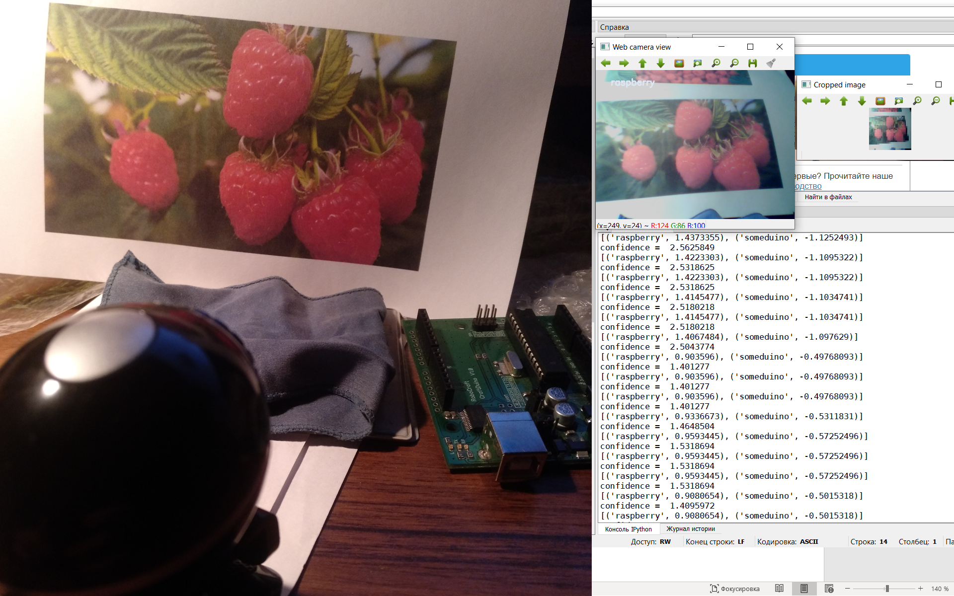
Detections is a vector in which the first number is the probability that our object can be attributed to the first class (raspberry), and the second number, respectively, to the second.



So let's see what we get.



To run this code, I used Spider, which is included with Anaconda. I also installed OpenCV 4th version.



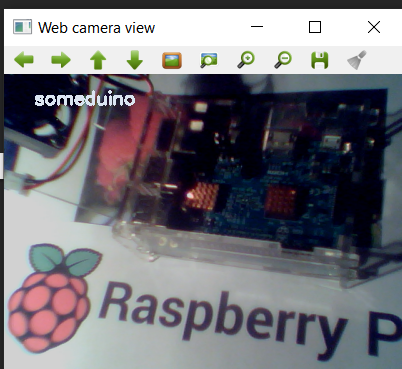
Let's start with Arduino.











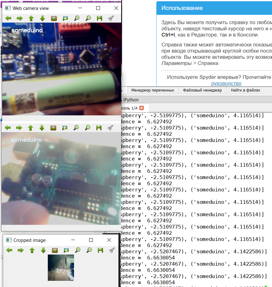
Since there were different types of Arduino-like devices in the training set, the model also recognizes CraftDuino v 1.0. and Arduino Nano, which my friend DrZugrik soldered to the board along with other components.



I don’t have live raspberries therefore we recognize photos from a leaflet (from the smartphone screen it is also possible).











So, our first model coped, let's see how the second copes.



The code for the second model is almost the same, except for the image conversion parameters. Therefore, we hide it under the spoiler.





Take my word that this model recognizes at least as well.



Therefore, we will prepare for her a more difficult task.



Namely, to recognize the Raspberry pi.







Well, everything is not so simple here, although it is quite expected, because “Though you call her a rose, though not”, despite her name, “Raspberry” looks more like Arduino.



Finally.



There is one big drawback in this solution, we chose the wrong model for recognition. Therefore, even if the camera looks into the void, it still tries to classify the object either as raspberry or as a controller.











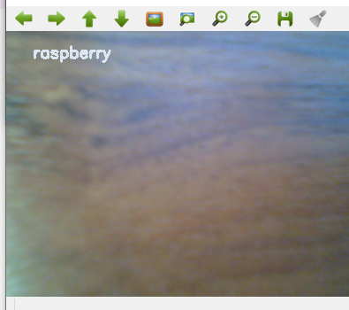
In order to recognize images with a colored frame, we need not only use models for classification, but models for recognition of objects in the image. But this is a completely different story, which I will write about a little later.