❓ ✌🏾 💻 Quantum trajectories and what they eat with 😕 🖖 🛷

This small note is about how to draw beautiful pictures, well, a little about physics, which is rarely talked about, about Bomov quantum mechanics.

Small introduction

As any science fiction and pseudoscientific nonsense likes to tell us, such as the movie The Secret, the laws of the microworld are very different from the classical ones that we are used to.

In the world of quantum mechanics, the probability given by the wave function rules everything.

p s i

$\ psi$ (those interested in details can look, for example, in the post “Muon catalysis from the point of view of quantum chemistry. Part I: ordinary hydrogen vs. muon hydrogen” ).

The legs of all kinds of funny things, such as Schrödinger cats , Heisenberg's uncertainty principles, and Bell's inequalities, grow out of the probabilistic properties of a quantummech.

But all these pictures with all kinds of electron orbitals did not answer the question “how does an electron fly in space”. To clarify this situation, physicists spent a lot of time, but could not cope with it. But David Bohm (known to many by the Aaronov-Bohm effect ) finally created one of the formalisms of quantum mechanics (name of himself) , in which there are still trajectories along which the quantum particle moves. And, unlike the Feynman path integrals , this path for each particle is exactly one. This property fundamentally allows you to track the movement of particles, and compare the motion of classical and quantum particles, which we will deal with in this article.

not only formalism

Actually, nobody is particularly interested in formalism itself, but from this formalism one can construct one of the interpretations of quantum mechanics, which, due to the seeming simplicity of classical mechanics, is loved by some freaks (not many, because it’s not very easy to enter this business).

We will not discuss this (as well as others) interpretation.

Classical and quantum trajectories

We will consider a rather boring system: one electron in the field of several protons. You can read about this system, as well as classical and quantum mechanics in the first and second parts of the posts “Muon catalysis from the point of view of quantum chemistry”.

The classical problem of particle motion in some potential is given by Newton's second law:

m d d o t x = F

$m \ ddot {x} = F$

where m is the particle mass, x is the coordinate, F is the force acting on the particle, and

d d o t x = f r a c d^{2} x d t^{2}

$\ ddot {x} = \ frac {d ^ 2 x} {dt ^ 2}$ - the second derivative of the particle’s coordinate in time, or acceleration. If only potential forces act in the system, then the force can be expressed through a new entity, potential energy V as

F = - f r a c d V d x

$F = - \ frac {dV} {dx}$

In our case, an electron in the field of several protons,

where the electron interacts with each of the protons according to Coulomb's law

V (R) = - k e^{2} / R

$V (R) = - k e ^ 2 / R$

, where k is the coefficient equal to 1 in atomic units, e is the charge of the electron, and R is the distance from the electron to the proton.

In this case, the total potential acting on the electron will be equal to

V = s u m_{n = 1}^{N} V_{n} (R_{n}) = - s u m_{n = 1}^{N} f r a c k e^{2} R_{n}

$V = \ sum_ {n = 1} ^ N V_n (R_n) = - \ sum_ {n = 1} ^ N \ frac {k e ^ 2} {R_n} \,$

where the index n numbers the protons (total protons N pieces), and R _n is the distance from the electron to the n- th proton.

Numerically solving the diffur, which is Newton’s second law, is a hackneyed task, the main thing is to set the initial position and speed. If the electron flies too fast, it will break out of the attraction of the proton (s) and fly off to infinity, and if there is just a bit of energy, it will forever flutter in the field of one of the nuclei, never visiting the others.

Radiant friction

If we took into account radiant friction , which arises due to the fact that when moving with acceleration, the electron would give part of its energy to the electromagnetic field, emitting it somewhere, then the electron would eventually roll onto the core in some time.

So what happens in the classics, we know.

But what will happen in the Bomov dynamics?

In this case, the particle will also move according to Newton’s second law with potential

V = V_{} m a t h r m C + V_{} m a t h r m Q

$V = V_ \ mathrm {C} + V_ \ mathrm {Q}$ where

V_{} m a t h r m C

$V_ \ mathrm {C}$ - the classical potential from the usual Newton's law, which in our case has the form given above.

Those. in addition to the classical potential, another entity will act on it: the quantum potential

V_{} m a t h r m Q

$V_ \ mathrm {Q}$ having (in 1D case) the form

V_{} m a t h r m Q = - f r a c h b a r^{2} 2 m A f r a c d^{2} A d x^{2}

$V_ \ mathrm {Q} = - \ frac {\ hbar ^ 2} {2mA} \ frac {d ^ 2A} {dx ^ 2}$

where A is the amplitude (modulus) of the wave function

A = | p s i |

$A = | \ psi |$ (

p s i = A e x p (i v a r p h i)

$\ psi = A \ exp (i \ varphi)$ where

v a r p h i

$\ varphi$ - phase of the wave function).

So, to get the equation of motion for a quantum particle, we still need to know something about the wave function.

About hidden options

Bohm's formalism is a theory with hidden parameters. But since the hidden parameter (wave function) is non-local, the calculation results in this formalism still satisfy Bell's aforementioned inequalities.

In the case of one proton, we know (see, for example, here ) the exact expression of the electron wave function in the ground (1s) state [ in atomic units ]:

p s i (R) = e x p (- R)

$\ psi (R) = \ exp (-R)$

About normalization and units

In the formula for the quantum potential, the normalization of the numerator will be reduced with the denominator, so we will not worry about it.

The argument of the exponent, in fact, is not worth

R

$R$ , but

R / a_{0}

$R / a_0$ where

a_{0}

$a_0$ Is the Bohr radius (0.529 Å). But, since we use atomic units, where

a_{0} = 1

$a_0 = 1$ , this unit of length we can afford not to write. You can read more about this here .

In the case of several protons, within the framework of the molecular orbitals method as combinations of atomic orbitals ( MO LKAO , see here ), the ground state with a sufficient degree of accuracy will be given by the sum of 1s-orbitals of each of the atoms:

p s i a p p r o x s u m_{n = 1}^{N} p s i_{n} (R_{n}) = s u m_{n = 1}^{N} e x p (- R_{n})

$\ psi \ approx \ sum_ {n = 1} ^ N \ psi_n (R_n) = \ sum_ {n = 1} ^ N \ exp (-R_n)$

Now, to find out the quantum potential, you just need to use this expression.

Well <s> d </s>

Function

p s i

$\ psi$ as the sum of 1s orbitals is real, therefore

A = p s i

$A = \ psi$ .

Since an electron can move in three dimensions, a one-dimensional derivative is needed

A_{x x}^{″} = f r a c d^{2} A d x^{2}

$A_ {xx} '' = \ frac {d ^ 2 A} {dx ^ 2}$ replace with its three-dimensional generalization:

D e l t a A = A_{x x}^{″} + A_{y y}^{″} + A_{z z}^{″}

$\ Delta A = A_ {xx} '' + A_ {yy} '' + A_ {zz} ''$ . Operator

D e l t a

$\ Delta$ can be represented as the square of the operator nabla :

D e l t a = n a b l a^{2}

$\ Delta = \ nabla ^ 2$ . You can also imagine the distance

R_{n}

$R_n$ as

R_{n} = s q r t m a t h b f R_{n}^{2}

$R_n = \ sqrt {\ mathbf {R} _n ^ 2}$ where

m a t h b f R_{n}

$\ mathbf {R} _n$ Is the radius vector of the electron relative to the nth proton.

Then

D e l t a A = n a b l a^{2} p s i = s u m_{n = 1}^{N} n a b l a^{2} p s i_{n} (R_{n})

$\ Delta A = \ nabla ^ 2 \ psi = \ sum_ {n = 1} ^ N \ nabla ^ 2 \ psi_n (R_n)$

The first derivative is considered easy:

n a b l a p s i_{n} (R_{n}) = n a b l a e x p (- R_{n}) = e x p (- R_{n}) c d o t (- 1) c d o t f r a c 1 2 u n d e r b r a c e {s q r t m a t h b f R_{n}^{2}}_{R_{n}} c d o t 2 m a t h b f R_{n} = - e x p (- R_{n}) c d o t f r a c m a t h b f R_{n} R_{n}

$\ nabla \ psi_n (R_n) = \ nabla \ exp (-R_n) = \ exp (-R_n) \ cdot (-1) \ cdot \ frac {1} {2 \ underbrace {\ sqrt {\ mathbf {R} _n ^ 2}} _ {R_n}} \ cdot 2 \ mathbf {R} _n = - \ exp (-R_n) \ cdot \ frac {\ mathbf {R} _n} {R_n}$

The second derivative is already somewhat more complicated:

n a b l a (n a b l a e x p (- R_{n})) = - f r a c m a t h b f R_{n} R_{n} n a b l a e x p (- R_{n}) - e x p (- R_{n}) n a b l a f r a c m a t h b f R_{n} R_{n} = e x p (- R_{n}) - f r a c 2 e x p (- R_{n}) R_{n}

$\ nabla (\ nabla \ exp (-R_n)) = - \ frac {\ mathbf {R} _n} {R_n} \ nabla \ exp (-R_n) - \ exp (-R_n) \ nabla \ frac {\ mathbf {R} _n} {R_n} = \ exp (-R_n) - \ frac {2 \ exp (-R_n)} {R_n}$

Where

- f r a c m a t h b f R_{n} R_{n} n a b l a e x p (- R_{n}) = e x p (- R_{n}) c d o t u n d e r b r a c e {l e f t (- f r a c m a t h b f R_{n} R_{n} r i g h t)^{2}}_{1} = e x p (- R_{n})

$- \ frac {\ mathbf {R} _n} {R_n} \ nabla \ exp (-R_n) = \ exp (-R_n) \ cdot \ underbrace {\ left (- \ frac {\ mathbf {R} _n} { R_n} \ right) ^ 2} _ {1} = \ exp (-R_n)$ and

- e x p (- R_{n}) n a b l a f r a c m a t h b f R_{n} R_{n} = - e x p (- R_{n}) c d o t l e f t (f r a c o v e r b r a c e {n a b l a m a t h b f R_{n}}^{3} R_{n} - f r a c 2 m a t h b f R_{n}^{2} 2 R_{n}^{3} r i g h t) = - f r a c 2 e x p (- R_{n}) R_{n}

$- \ exp (-R_n) \ nabla \ frac {\ mathbf {R} _n} {R_n} = - \ exp (-R_n) \ cdot \ left (\ frac {\ overbrace {\ nabla \ mathbf {R} _n } ^ {3}} {R_n} - \ frac {2 \ mathbf {R} _n ^ 2} {2 R_n ^ 3} \ right) = - \ frac {2 \ exp (-R_n)} {R_n}$ .

The result remains:

D e l t a p s i = o v e r b r a c e {s u m_{n = 1}^{N} e x p (- R_{n})}^{p s i} - s u m_{n = 1}^{N} f r a c 2 e x p (- R_{n}) R_{n}

$\ Delta \ psi = \ overbrace {\ sum_ {n = 1} ^ {N} \ exp (-R_n)} ^ {\ psi} - \ sum_ {n = 1} ^ {N} \ frac {2 \ exp (-R_n)} {R_n}$

Dividing everything into

p s i = A

$\ psi = A$ and multiplying by

- f r a c h b a r^{2} 2 m

$- \ frac {\ hbar ^ 2} {2m}$

we get

V_{} m a t h r m Q = - f r a c h b a r^{2} 2 m l e f t (1 - s u m_{n = 1}^{N} f r a c 2 e x p (- R_{n}) R_{n} r i g h t)

$V_ \ mathrm {Q} = - \ frac {\ hbar ^ 2} {2m} \ left (1 - \ sum_ {n = 1} ^ N \ frac {2 \ exp (-R_n)} {R_n} \ right )$

The unit in the differentiation to obtain power will disappear, so you can safely leave only the second term.

As a result, we can write down our quantum potential as

V_{} m a t h r m Q a p p r o x f r a c h b a r^{2} m s u m_{n = 1}^{N} f r a c e x p (- R_{n}) R_{n}

$V_ \ mathrm {Q} \ approx \ frac {\ hbar ^ 2} {m} \ sum_ {n = 1} ^ N \ frac {\ exp (-R_n)} {R_n}$

and with this expression we can already drive the Bohm dynamics of an electron in the field of many protons.

Implementation

For all this disgrace, code was written in python, it is available here:

Python code

from math import * import numpy as np cutoff=5.0e-4 Quantum=True def dist(r1,r2): return np.dot((r1-r2), (r1-r2)) def Vc(r, r0): if dist(r, r0)>=cutoff: return -1.0/dist(r, r0) else: return -1.0/cutoff rH=[] #h1 #rH.append(np.array([ 0.0, 0.0, 0.0])) #h2 rH.append(np.array([-1.0, 0.0, 0.0])) rH.append(np.array([+1.0, 0.0, 0.0])) def Vat(r): V=0.0 for rh in rH: V+=Vc(r,rh) return V def PsiA(r): psi=0.0 for rh in rH: if dist(r, rh)<1.0e3: psi+=np.exp(-dist(r, rh)) return psi def Vq(r): vq=0.0 for rh in rH: if dist(r, rh)>=cutoff: vq-=2.0*np.exp(-dist(r, rh))/dist(r, rh) else: vq-=2.0*np.exp(-cutoff)/cutoff vq*=(-0.5) # -0.5*hbar**2/me return vq def GradF(F, r): grad=np.zeros(3) dx=0.1 for i in range(0,3): dr=np.zeros(3) dr[i]=dx #print(dr) #print(F(r+dr)-F(r-dr)) grad[i]+=(F(r+dr)-F(r-dr))/(2.*dx) return grad dt=0.001 tmax=2.0e1 DR=1.0 dx=0.001 MaxR=10.0 t=0.0 cent=np.zeros(3) Ntrj=30 m=1.0 def GenRvBox(DX): return np.random.uniform(-DX,+DX,3) def GenRvSph(DX): r=np.random.uniform(0.0,DX) phi=np.random.uniform(0.0,2.0*np.pi) theta=np.random.uniform(0.0,np.pi) x=r*np.sin(theta)*np.cos(phi) y=r*np.sin(theta)*np.sin(phi) z=r*np.cos(theta) return np.array([x,y,z]) for ntrj in range(0,Ntrj): if Quantum: outf=open("bmd_%05i" % (ntrj) + ".trj", "w") else: outf=open("cmd_%05i" % (ntrj) + ".trj", "w") nat=np.random.randint(0,len(rH)) r=rH[nat]+GenRvSph(DR) rprev=r+GenRvBox(dx) outf.write("%15.10f %15.10f %15.10f\n" % tuple(r)) t=0.0 while t<=tmax and dist(r,cent)<=MaxR: F= -GradF(Vat, r) if Quantum: F-= GradF(Vq, r) rnew= 2.*r - rprev + (F/m)*dt**2 rprev=r r=rnew outf.write("%15.10f %15.10f %15.10f\n" % tuple(r)) t+=dt outf.close() exit()

We will only discuss a few points.

Newton’s second law is integrated using the Verlet algorithm :

x (t + D e l t a t) = 2 x (t) - x (t - D e l t a t) + f r a c F (t) m D e l t a t^{2}

$x (t + \ Delta t) = 2 x (t) - x (t - \ Delta t) + \ frac {F (t)} {m} \ Delta t ^ 2$

The initial position is generated by randomly selecting one of the protons, a direction is randomly selected around it (using spherical coordinates). To set the initial speed, you need to set another, previous position. It is selected using another small random vector.

Turning on / off the quantum potential, we switch to quantum / classical modes of motion.

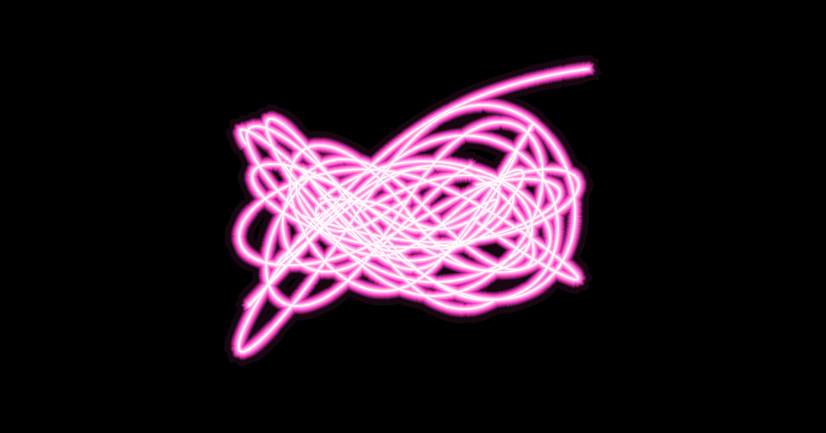
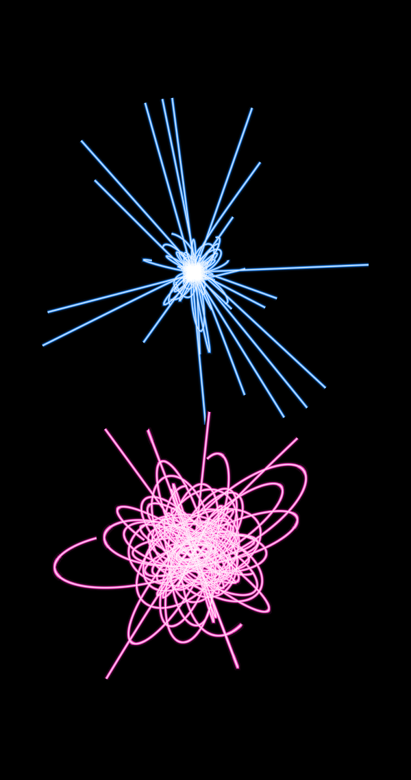
Well, then, you can build beautiful pictures using Gnuplot for the hydrogen atom

and for the molecule H ₂ ⁺

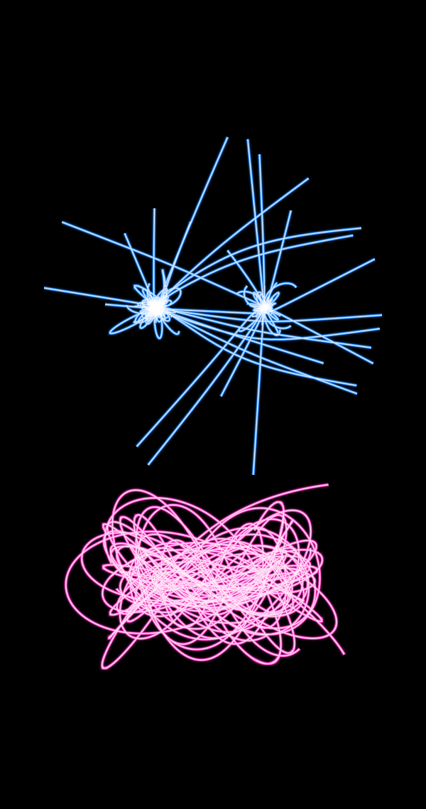
As you can see, the classical trajectories (upper, blue) are either very localized, or if the electron is forced to move too quickly, they run away from the nuclei. In the quantum case (lower, pink), the quantum potential allows the electrons to walk significantly farther from the nucleus, and in the case of the H2 ⁺ molecule, it allows you to run from one proton to another, which is an indirect visualization of chemical bonds.

A few words about building pictures: to create a neon effect, each path is drawn many times, from thin white to thick black, through the shadows of the color of interest. For the convenience of choosing such a palette, you can, for example, use the site https://www.color-hex.com/

An example script is given below.

Script for Gnuplot

unset key 
      

        
        
        
      

     set xyplane relative 0 
      

        
        
        
      

     
      

        
        
        
      

     unset box 
      

        
        
        
      

     
      

        
        
        
      

     set view map 
      

        
        
        
      

     
      

        
        
        
      

     set size ratio -1 
      

        
        
        
      

     
      

        
        
        
      

     unset border 
      

        
        
        
      

     unset xtics 
      

        
        
        
      

     unset ytics 
      

        
        
        
      

     
      

        
        
        
      

     set terminal pngcairo size 2160,4096 backgr rgb "black" 
      

        
        
        
      

     set output "tmp.png" 
      

        
        
        
      

     
      

        
        
        
      

     yshift=-5.0 
      

        
        
        
      

     maxiC=29 
      

        
        
        
      

     maxiQ=29 
      

        
        
        
      

     splot \ 
      

        
        
        
      

     for [i=0:maxiC] sprintf("cmd_%05i.trj", i) wl lw 30.0 lc rgb "#030d19" not,\ 
      

        
        
        
      

     for [i=0:maxiC] sprintf("cmd_%05i.trj", i) wl lw 18.0 lc rgb "#071b33" not,\ 
      

        
        
        
      

     for [i=0:maxiC] sprintf("cmd_%05i.trj", i) wl lw 17.0 lc rgb "#0a294c" not,\ 
      

        
        
        
      

     for [i=0:maxiC] sprintf("cmd_%05i.trj", i) wl lw 16.0 lc rgb "#0e3766" not,\ 
      

        
        
        
      

     for [i=0:maxiC] sprintf("cmd_%05i.trj", i) wl lw 15.0 lc rgb "#11457f" not,\ 
      

        
        
        
      

     for [i=0:maxiC] sprintf("cmd_%05i.trj", i) wl lw 14.0 lc rgb "#155399" not,\ 
      

        
        
        
      

     for [i=0:maxiC] sprintf("cmd_%05i.trj", i) wl lw 13.0 lc rgb "#1861b2" not,\ 
      

        
        
        
      

     for [i=0:maxiC] sprintf("cmd_%05i.trj", i) wl lw 12.0 lc rgb "#1c6fcc" not,\ 
      

        
        
        
      

     for [i=0:maxiC] sprintf("cmd_%05i.trj", i) wl lw 11.0 lc rgb "#1f7de5" not,\ 
      

        
        
        
      

     for [i=0:maxiC] sprintf("cmd_%05i.trj", i) wl lw 10.0 lc rgb "#238bff" not,\ 
      

        
        
        
      

     for [i=0:maxiC] sprintf("cmd_%05i.trj", i) wl lw 9.0 lc rgb "#3896ff" not,\ 
      

        
        
        
      

     for [i=0:maxiC] sprintf("cmd_%05i.trj", i) wl lw 8. lc rgb "#4ea2ff" not,\ 
      

        
        
        
      

     for [i=0:maxiC] sprintf("cmd_%05i.trj", i) wl lw 7. lc rgb "#65adff" not,\ 
      

        
        
        
      

     for [i=0:maxiC] sprintf("cmd_%05i.trj", i) wl lw 6. lc rgb "#7bb9ff" not,\ 
      

        
        
        
      

     for [i=0:maxiC] sprintf("cmd_%05i.trj", i) wl lw 5. lc rgb "#91c5ff" not,\ 
      

        
        
        
      

     for [i=0:maxiC] sprintf("cmd_%05i.trj", i) wl lw 4. lc rgb "#a7d0ff" not,\ 
      

        
        
        
      

     for [i=0:maxiC] sprintf("cmd_%05i.trj", i) wl lw 3. lc rgb "#bddcff" not,\ 
      

        
        
        
      

     for [i=0:maxiC] sprintf("cmd_%05i.trj", i) wl lw 2. lc rgb "#d3e7ff" not,\ 
      

        
        
        
      

     for [i=0:maxiC] sprintf("cmd_%05i.trj", i) wl lw 1. lc rgb "#e9f3ff" not,\ 
      

        
        
        
      

     for [i=0:maxiC] sprintf("cmd_%05i.trj", i) wl lw 0.5 lc rgb "#ffffff" not,\ 
      

        
        
        
      

     for [i=0:maxiQ] sprintf("bmd_%05i.trj", i) u 1:($2+yshift):3 wl lw 30.0 lc rgb "#190613" not,\ 
      

        
        
        
      

     for [i=0:maxiQ] sprintf("bmd_%05i.trj", i) u 1:($2+yshift):3 wl lw 18.0 lc rgb "#330c27" not,\ 
      

        
        
        
      

     for [i=0:maxiQ] sprintf("bmd_%05i.trj", i) u 1:($2+yshift):3 wl lw 17.0 lc rgb "#4c123b" not,\ 
      

        
        
        
      

     for [i=0:maxiQ] sprintf("bmd_%05i.trj", i) u 1:($2+yshift):3 wl lw 16.0 lc rgb "#66184f" not,\ 
      

        
        
        
      

     for [i=0:maxiQ] sprintf("bmd_%05i.trj", i) u 1:($2+yshift):3 wl lw 15.0 lc rgb "#7f1e63" not,\ 
      

        
        
        
      

     for [i=0:maxiQ] sprintf("bmd_%05i.trj", i) u 1:($2+yshift):3 wl lw 14.0 lc rgb "#992476" not,\ 
      

        
        
        
      

     for [i=0:maxiQ] sprintf("bmd_%05i.trj", i) u 1:($2+yshift):3 wl lw 13.0 lc rgb "#b22a8a" not,\ 
      

        
        
        
      

     for [i=0:maxiQ] sprintf("bmd_%05i.trj", i) u 1:($2+yshift):3 wl lw 12.0 lc rgb "#cc309e" not,\ 
      

        
        
        
      

     for [i=0:maxiQ] sprintf("bmd_%05i.trj", i) u 1:($2+yshift):3 wl lw 11.0 lc rgb "#e536b2" not,\ 
      

        
        
        
      

     for [i=0:maxiQ] sprintf("bmd_%05i.trj", i) u 1:($2+yshift):3 wl lw 10.0 lc rgb "#ff3dc6" not,\ 
      

        
        
        
      

     for [i=0:maxiQ] sprintf("bmd_%05i.trj", i) u 1:($2+yshift):3 wl lw 9.0 lc rgb "#ff50cb" not,\ 
      

        
        
        
      

     for [i=0:maxiQ] sprintf("bmd_%05i.trj", i) u 1:($2+yshift):3 wl lw 8. lc rgb "#ff63d1" not,\ 
      

        
        
        
      

     for [i=0:maxiQ] sprintf("bmd_%05i.trj", i) u 1:($2+yshift):3 wl lw 7. lc rgb "#ff77d7" not,\ 
      

        
        
        
      

     for [i=0:maxiQ] sprintf("bmd_%05i.trj", i) u 1:($2+yshift):3 wl lw 6. lc rgb "#ff8adc" not,\ 
      

        
        
        
      

     for [i=0:maxiQ] sprintf("bmd_%05i.trj", i) u 1:($2+yshift):3 wl lw 5. lc rgb "#ff9ee2" not,\ 
      

        
        
        
      

     for [i=0:maxiQ] sprintf("bmd_%05i.trj", i) u 1:($2+yshift):3 wl lw 4. lc rgb "#ffb1e8" not,\ 
      

        
        
        
      

     for [i=0:maxiQ] sprintf("bmd_%05i.trj", i) u 1:($2+yshift):3 wl lw 3. lc rgb "#ffc4ed" not,\ 
      

        
        
        
      

     for [i=0:maxiQ] sprintf("bmd_%05i.trj", i) u 1:($2+yshift):3 wl lw 2. lc rgb "#ffd8f3" not,\ 
      

        
        
        
      

     for [i=0:maxiQ] sprintf("bmd_%05i.trj", i) u 1:($2+yshift):3 wl lw 1. lc rgb "#ffebf9" not,\ 
      

        
        
        
      

     for [i=0:maxiQ] sprintf("bmd_%05i.trj", i) u 1:($2+yshift):3 wl lw 0.5 lc rgb "#ffffff" not

Conclusion

The Bomov trajectories, although difficult to understand and calculate, allow you to draw beautiful pictures that show how much more fun and richer than classical mechanics.

If you have comments, questions, suggestions: write. :)

Quantum trajectories and what they eat with

Small introduction

Classical and quantum trajectories

Implementation

Conclusion

More articles: