Having come across an article “ Destroying the monopoly ... ”, the author, as a person, albeit very distant from EDA , but naturally inquisitive, was not too lazy to follow the links and involuntarily caught himself thinking that one of the main technical solutions is the use of rows of standard cells ( standard cell layout) - looks pretty controversial.
Yes, this arrangement is intuitive, because we write and read in a similar way, in addition, it is technologically simple to arrange cells in rows, it is so convenient to connect the VDD and GND buses. On the other hand, a complex combinatorial problem arises, it is necessary to cut the circuit into linear pieces and arrange these pieces in such a way as to (roughly) minimize the total length of the joints.
And of course, the question arose of whether there are alternative solutions ... that’s what if ...

Figure 1 typical rows of standard cells ( from here )
What if
From the point of view of reducing the total bond length, it would be useful to arrange standard cells along some of the sweeping ex curves : Peano or Hilbert.
These curves consist of a mass of various “nooks and crannies,” for sure there is a configuration in which the connected standard cells are on average close to each other.
Or it can serve as a zero iteration for further optimization.
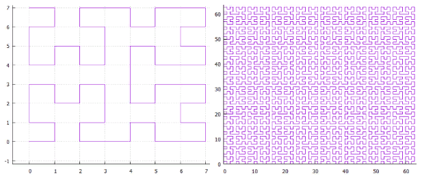
Figure 2 Hilbert curve, fields 8X8 and 64X64
- The sweeping curves are self-similar, which fits well into the overall concept.
- They have a high locality i.e. points located somewhere nearby on the curve are most likely nearby and in space.
- Contain a hierarchically organized network of channels.
- For the logical circuit, you can choose a suitable square or rectangle 1x2,2x1 in which it is placed in excess and "move" it along the sweeping curve (see Figure 3) to choose the optimal geometry, because this is only one degree of freedom with a rather cheap cost function .
- Convenience of connection of tires (VDD / GND) will remain.
- ...

Figure 3 Three pieces of a Hilbert curve with different shifts.
So:
- we will experiment with the Hilbert curve
- we will experiment in a square 64X64 (Figure 3)
- in the elementary step of the curve there can be several standard cells and spaces - how many and in what order - the parameter of the experiment
- all elementary steps are arranged identically
- elementary steps go with an overlap i.e. if the step begins with a standard cell, there must be a space at the end of it, and vice versa
- all spaces and standard cells are the same size - 1X1
- all cells are serialized in some order, this order is also a parameter
- one more parameter is the shift from the beginning of the curve (points (0,0)), starting from which we will arrange the standard cells in a certain order
- bond lengths between standard cells are calculated according to L1 (Manhattan distance)
- the sum of the lengths of all bonds is the desired value, having determined the minimum amount, we will find the optimal location
And as an experimental rabbit, let's take an 8-bit adder. It is simple enough, but not trivial. There are a lot of elements and connections in it to feel the potential pros and cons. At the same time, there are not enough of them to be able to experiment “on the knee”.
Adder

4 is a schematic diagram of a full single-bit adder

Figure 5 So sees this graph utility Neato from graphwiz

6 8-bit signed adder, taken here
But we will only work with integers, without the error flag W.
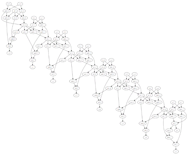
Fig. 7 So the 8-bit adder sees the dot utility of graphwiz.
It looks like a dance of little swans.

Fig. 8 is the same graph after optimization using neato.
DOT Count
digraph sum8 {
a_0;
a_1;
a_2;
a_3;
a_4;
a_5;
a_6;
a_7;
b_0;
b_1;
b_2;
b_3;
b_4;
b_5;
b_6;
b_7;
s_0;
s_1;
s_2;
s_3;
s_4;
s_5;
s_6;
s_7;
p0;
p1;
and1_0;
and1_1;
and1_2;
and1_3;
and1_4;
and1_5;
and1_6;
and1_7;
and2_0;
and2_1;
and2_2;
and2_3;
and2_4;
and2_5;
and2_6;
and2_7;
and3_0;
and3_1;
and3_2;
and3_3;
and3_4;
and3_5;
and3_6;
and3_7;
and4_0;
and4_1;
and4_2;
and4_3;
and4_4;
and4_5;
and4_6;
and4_7;
or1_0;
or1_1;
or1_2;
or1_3;
or1_4;
or1_5;
or1_6;
or1_7;
or2_0;
or2_1;
or2_2;
or2_3;
or2_4;
or2_5;
or2_6;
or2_7;
or3_0;
or3_1;
or3_2;
or3_3;
or3_4;
or3_5;
or3_6;
or3_7;
or4_0;
or4_1;
or4_2;
or4_3;
or4_4;
or4_5;
or4_6;
or4_7;
not1_0;
not1_1;
not1_2;
not1_3;
not1_4;
not1_5;
not1_6;
not1_7;
a_0 -> and1_0;
a_1 -> and1_1;
a_2 -> and1_2;
a_3 -> and1_3;
a_4 -> and1_4;
a_5 -> and1_5;
a_6 -> and1_6;
a_7 -> and1_7;
b_0 -> and1_0;
b_1 -> and1_1;
b_2 -> and1_2;
b_3 -> and1_3;
b_4 -> and1_4;
b_5 -> and1_5;
b_6 -> and1_6;
b_7 -> and1_7;
a_0 -> or1_0;
a_1 -> or1_1;
a_2 -> or1_2;
a_3 -> or1_3;
a_4 -> or1_4;
a_5 -> or1_5;
a_6 -> or1_6;
a_7 -> or1_7;
b_0 -> or1_0;
b_1 -> or1_1;
b_2 -> or1_2;
b_3 -> or1_3;
b_4 -> or1_4;
b_5 -> or1_5;
b_6 -> or1_6;
b_7 -> or1_7;
and1_0 -> or3_0;
and1_1 -> or3_1;
and1_2 -> or3_2;
and1_3 -> or3_3;
and1_4 -> or3_4;
and1_5 -> or3_5;
and1_6 -> or3_6;
and1_7 -> or3_7;
and1_0 -> and3_0;
and1_1 -> and3_1;
and1_2 -> and3_2;
and1_3 -> and3_3;
and1_4 -> and3_4;
and1_5 -> and3_5;
and1_6 -> and3_6;
and1_7 -> and3_7;
or1_0 -> and2_0;
or1_1 -> and2_1;
or1_2 -> and2_2;
or1_3 -> and2_3;
or1_4 -> and2_4;
or1_5 -> and2_5;
or1_6 -> and2_6;
or1_7 -> and2_7;
or1_0 -> or2_0;
or1_1 -> or2_1;
or1_2 -> or2_2;
or1_3 -> or2_3;
or1_4 -> or2_4;
or1_5 -> or2_5;
or1_6 -> or2_6;
or1_7 -> or2_7;
and2_0 -> or3_0;
and2_1 -> or3_1;
and2_2 -> or3_2;
and2_3 -> or3_3;
and2_4 -> or3_4;
and2_5 -> or3_5;
and2_6 -> or3_6;
and2_7 -> or3_7;
or2_0 -> and4_0;
or2_1 -> and4_1;
or2_2 -> and4_2;
or2_3 -> and4_3;
or2_4 -> and4_4;
or2_5 -> and4_5;
or2_6 -> and4_6;
or2_7 -> and4_7;
and3_0 -> or4_0;
and3_1 -> or4_1;
and3_2 -> or4_2;
and3_3 -> or4_3;
and3_4 -> or4_4;
and3_5 -> or4_5;
and3_6 -> or4_6;
and3_7 -> or4_7;
or3_0 -> not1_0;
or3_1 -> not1_1;
or3_2 -> not1_2;
or3_3 -> not1_3;
or3_4 -> not1_4;
or3_5 -> not1_5;
or3_6 -> not1_6;
or3_7 -> not1_7;
not1_0 -> and4_0;
not1_1 -> and4_1;
not1_2 -> and4_2;
not1_3 -> and4_3;
not1_4 -> and4_4;
not1_5 -> and4_5;
not1_6 -> and4_6;
not1_7 -> and4_7;
and4_0 -> or4_0;
and4_1 -> or4_1;
and4_2 -> or4_2;
and4_3 -> or4_3;
and4_4 -> or4_4;
and4_5 -> or4_5;
and4_6 -> or4_6;
and4_7 -> or4_7;
or4_0 -> s_0;
or4_1 -> s_1;
or4_2 -> s_2;
or4_3 -> s_3;
or4_4 -> s_4;
or4_5 -> s_5;
or4_6 -> s_6;
or4_7 -> s_7;
p0 -> and2_0;
p0 -> or2_0;
p0 -> and3_0;
or3_0 -> and2_1;
or3_0 -> or2_1;
or3_0 -> and3_1;
or3_1 -> and2_2;
or3_1 -> or2_2;
or3_1 -> and3_2;
or3_2 -> and2_3;
or3_2 -> or2_3;
or3_2 -> and3_3;
or3_3 -> and2_4;
or3_3 -> or2_4;
or3_3 -> and3_4;
or3_4 -> and2_5;
or3_4 -> or2_5;
or3_4 -> and3_5;
or3_5 -> and2_6;
or3_5 -> or2_6;
or3_5 -> and3_6;
or3_6 -> and2_7;
or3_6 -> or2_7;
or3_6 -> and3_7;
or3_7 -> p1;
}
Experiment 1
- elementary step of the Hilbert curve - (skip, cell, cell, skip)
- graph vertices (unit cells) sorted alphabetically
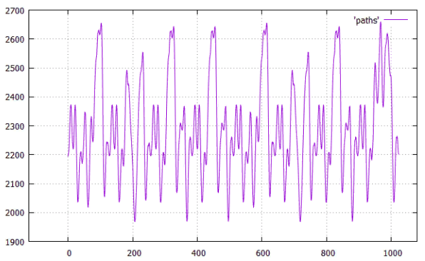
Fig.9 on X - shift from the beginning, on Y - the length of all paths
The minimum distance (the first of) at a shift of 207 (The total length of all bonds is 1968), let's see what this optimal arrangement looks like.

Figure 10 is the optimal graph for the shift 207, it does not look very nice.
Experiment 2
- elementary step of the Hilbert curve - (skip, cell, cell, skip)
- the vertices of the graph (unit cells) in the natural order (as came in the description of the graph, see the description of the graph above) -

11 on X - the shift from the beginning, on Y - the length of all paths
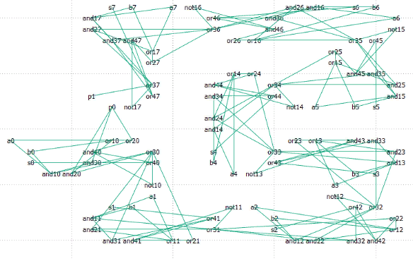
Fig. 12 optimal graph for shear 11 length 750
Experiment 3
- elementary step of the Hilbert curve - (skip, cell, cell, skip)
- the order of the vertices is determined by traversing the width of the graph, vertices without links at the beginning of the list, the weekend at the end

Fig.13 on X - shift from the beginning, on Y - the length of all paths
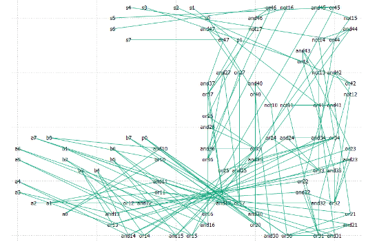
Fig. 14 Optimal arrangement — shift 3, total length 1451
Put all input vertices at the beginning, and output at the end was not very good
an idea.
Experiment 4
- the elementary step of the Hilbert curve - (pass, cell, cell) Sic!
- the vertex order is natural, as in experiment 2

Fig.15 on X - shift from the beginning, on Y - the length of all paths

Fig. 16 Optimal arrangement - shift 10, total length 503
Experiment 5
We need to do something with IO, we define them in post-processing, i.e. for each shift
construct an arrangement without IO vertices, then construct an absorbent extent frame around the graph, apply IO vertices to the nearest unoccupied point of the frame and calculate the final length
- elementary step of the Hilbert curve - (skip, cell, cell)
- the order of the vertices is determined by viewing in width, but without IO vertices

Fig.17 on X - shift from the beginning, on Y - the length of all paths
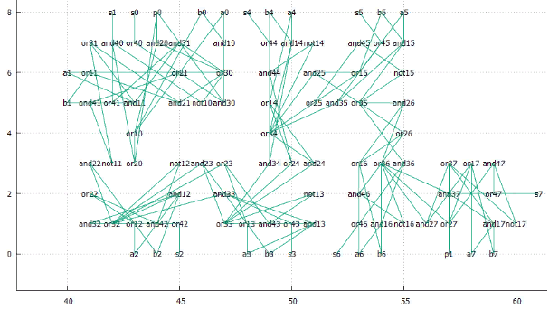
Fig. 18 The optimal location is the shift 607, the total length of 484, the average 3.33793
It looks good, but what if we optimize not the total length of the paths, but its sum with the area of the occupied rectangle. Their dimensions are different, so we assume that we calculate not the path length, but the area under the paths.
Experiment 6
The parameters are the same as in experiment 5, we optimize the area.
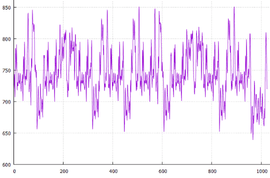
Fig.19 on X - shift from the beginning, on Y - the length of all paths
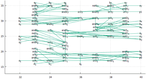
Fig. 20 Optimal arrangement - shift 966, total length 639, average 3.30345
The rectangle turned out quite elongated. But what if we consider not the area of the rectangle, but the square of the hypotenuse, pushing us to more square shapes?
Experiment 7
The parameters are the same as in experiment 5, we optimize the square of the hypotenuse.

Fig.21 on X is the shift from the beginning, on Y is the length of all paths

Fig. 22 Optimal arrangement - shift 70, total length 702, average 3.46207
Experiment 8
- elementary step of the Hilbert curve - (cell, skip) Sic!
- the order of the vertices is determined by viewing in width, but without IO vertices
We assume that the cost of walking in Y is twice as much as in X, this is closer to reality.
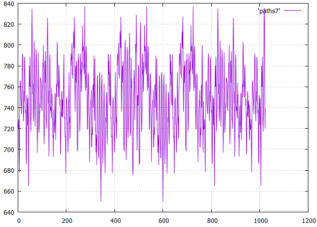
Fig.23 on X is the shift from the beginning, on Y is the length of all paths

Fig. 24 Optimal arrangement - shift 344, total length 650, average 3.8
conclusions
Preliminary “Editors' Choice” - Experiment 6.
It would be nice to arrange the IO vertices, but for this you need a hint from the side,
where exactly (direction) this class of vertices should be located.
But first I would like to hear the opinion of experts.
PS : thanks to YuriPanchul and andy_p for the lack of a reflex negative reaction.
UPD (11/02/2019): added “experiment 8”, where the standard cells are located at the nodes of the Hilbert curve, i.e. strictly on a square lattice. At the same time, they are united on the one hand in traditional series, and on the other hand, are located along the Hilbert curve.