On the Data tab, you can read the description of all fields.
All source code is in laptop format here .
We load the data, check that we generally have:
import numpy as np import pandas as pd dataset = pd.read_csv('../input/ghouls-goblins-and-ghosts-boo/train.csv') # X_test = pd.read_csv('../input/ghouls-goblins-and-ghosts-boo/test.csv') # print(dataset.shape) print(dataset[:10])
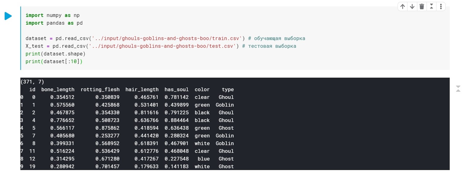
The values of the type field (Ghoul, Ghost, Goblin) are simply replaced by 0, 1 and 2.
Color - it is also necessary to pre-process it (we only need numerical values to build the model). We will use LabelEncoder and OneHotEncoder for this. More details .
from sklearn.preprocessing import LabelEncoder, OneHotEncoder labelencoder_X_1 = LabelEncoder() X_train[:, 4] = labelencoder_X_1.fit_transform(X_train[:, 4]) labelencoder_X_2 = LabelEncoder() X_test[:, 4] = labelencoder_X_2.fit_transform(X_test[:, 4]) labelencoder_Y_2 = LabelEncoder() Y_train = labelencoder_Y_2.fit_transform(Y_train) one_hot_encoder = OneHotEncoder(categorical_features = [4]) X_train = one_hot_encoder.fit_transform(X_train).toarray() X_test = one_hot_encoder.fit_transform(X_test).toarray()
Well, at this point our data is ready. It remains to train our model.
First apply Adagrad :
In essence, this is a modification of stochastic gradient descent, about which I wrote last time: habr.com/en/post/472300
This method takes into account the history of all past gradients for each individual parameter (the idea of scaling). This allows you to reduce the learning step size for parameters that have a large gradient:

g is the scaling parameter (g0 = 0)
θ - parameter (weight)
epsilon is a small constant introduced in order to prevent division by zero
Divide the dataset into 2 parts:
Training sample (train) and validation (val):
from sklearn.model_selection import train_test_split x_train, x_val, y_train, y_val = train_test_split(X_train, Y_train, test_size = 0.2)
A little preparation for model training:
import torch import numpy as np device = 'cuda' if torch.cuda.is_available() else 'cpu' def make_train_step(model, loss_fn, optimizer): def train_step(x, y): model.train() yhat = model(x) loss = loss_fn(yhat, y) loss.backward() optimizer.step() optimizer.zero_grad() return loss.item() return train_step
Self training model:
from torch import optim, nn model = torch.nn.Sequential( nn.Linear(10, 270), nn.ReLU(), nn.Linear(270, 3)) lr = 0.01 n_epochs = 500 loss_fn = torch.nn.CrossEntropyLoss() optimizer = optim.Adagrad(model.parameters(), lr=lr) train_step = make_train_step(model, loss_fn, optimizer) from sklearn.utils import shuffle for epoch in range(n_epochs): x_train, y_train = shuffle(x_train, y_train) # X = torch.FloatTensor(x_train) y = torch.LongTensor(y_train) loss = train_step(X, y) print(loss)
Model Rating:
# : test_var = torch.FloatTensor(x_val) with torch.no_grad(): result = model(test_var) values, labels = torch.max(result, 1) num_right = np.sum(labels.data.numpy() == y_val) print(' {:.2f}'.format(num_right / len(y_val)))
Here, in addition to layers, we have only 2 configurable parameters (for now):
learning rate and n_epochs (number of eras).
Depending on how we combine these two parameters, 3 situations may arise:
1 - everything is fine, i.e. the model shows low loss on the training sample and high accuracy on the validation one.
2 - underfitting - large loss on the training set and low accuracy on the validation one.
3 - overfitting - low loss on the training sample, but low accuracy on the validation.
With the first, everything is clear :)
With the second, it seems, too - to experiment with the learning rate and the n_epochs.
And what to do with the third? The answer is simple - regularization!
Previously, we had a loss function of the form:
L = MSE (Y, y) without additional terms
The essence of regularization consists precisely in adding a term to the objective function to “fine” the gradient if it is too large. In other words, we impose a restriction on our objective function.
There are many regularization methods. More about L1 and L2 - regularization: craftappmobile.com/l1-vs-l2-regularization/#_L1_L2
The Adagrad method implements L2 regularization, let's apply it!
First, for clarity, look at the indicators of the model without regularization:
lr = 0.01, n_epochs = 500:
loss = 0.44 ...
Accuracy: 0.71
lr = 0.01, n_epochs = 1000:
loss = 0.41 ...
Accuracy: 0.75
lr = 0.01, n_epochs = 2000:
loss = 0.39 ...
Accuracy: 0.75
lr = 0.01, n_epochs = 3000:
loss = 0.367 ...
Accuracy: 0.76
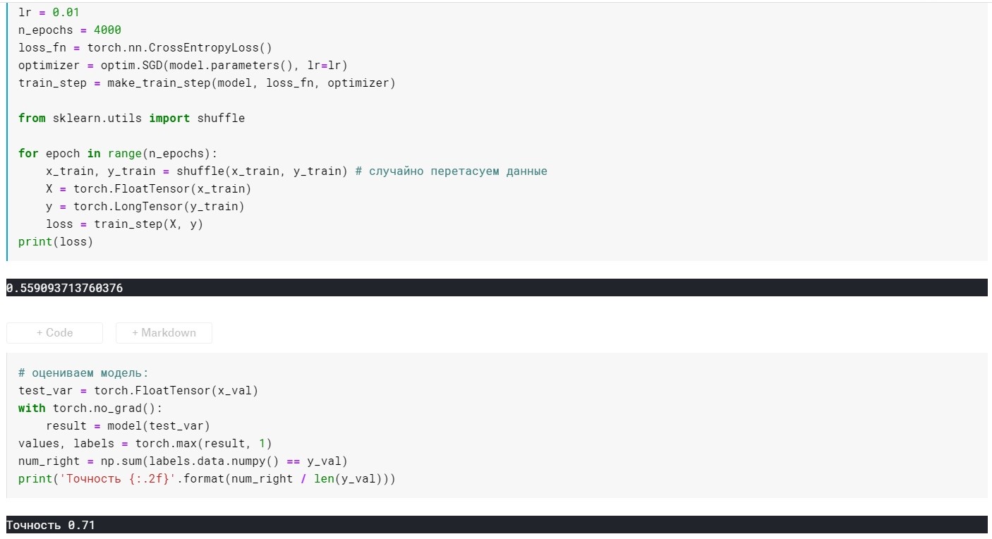
lr = 0.01, n_epochs = 4000:
loss = 0.355 ...
Accuracy: 0.72
lr = 0.01, n_epochs = 10000:
loss = 0.285 ...
Accuracy: 0.69
Here you can see that with 4k + eras - the model is already overfit. Now try to avoid this:
To do this, add the weight_decay parameter for our optimization method:
optimizer = optim.Adagrad(model.parameters(), lr=lr, weight_decay = 0.001)
With lr = 0.01, m_epochs = 10000:
loss = 0.367 ...
Accuracy: 0.73
At 4000 eras:
loss = 0.389 ...
Accuracy: 0.75
It turned out much better, but we added only 1 parameter in the optimizer :)
Now consider SGDm (this is a stochastic gradient descent with a small extension - heuristics, if you like).
The bottom line is that SGD updates the parameters quite strongly after each iteration. It would be logical to “smooth” the gradient, using gradients from previous iterations (the idea of inertia):

θ - parameter (weight)
µ - inertia hyperparameter
SGD without momentum parameter:
SGD with momentum parameter:
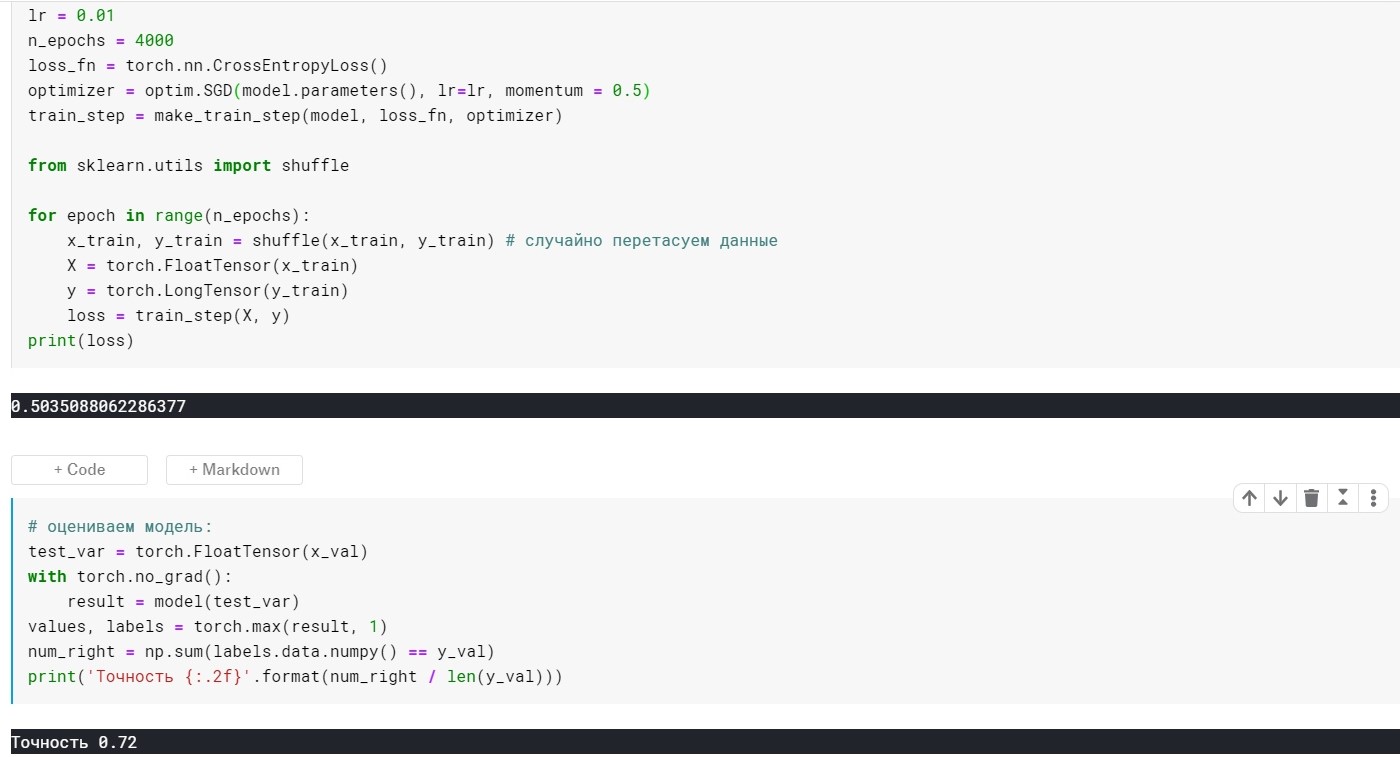
It turned out not much better, but the point here is that there are methods that immediately use the ideas of scaling and inertia. For example, Adam or Adadelta, which now show good results. Well, in order to understand these methods, I think it is necessary to understand some basic ideas used in simpler methods.
Thank you all for your attention!