We analyze the tonality of texts using Fast.ai

The article will discuss the classification of tonality of text messages in Russian (and essentially any classification of texts using the same technologies). We will take this article as a basis, in which the classification of tonality on the CNN architecture using the Word2vec model was considered. In our example, we will solve the same problem of separating tweets into positive and negative on the same dataset using the ULMFit model. The result from the article (average F1-score = 0.78142) will be accepted as a baseline.

Introduction

The ULMFIT model was introduced by fast.ai developers (Jeremy Howard, Sebastian Ruder) in 2018. The essence of the approach is to use transfer learning in NLP tasks when you use pre-trained models, reducing the time for training your models and reducing the requirements for the size of the labeled test sample.



The training scheme in our case will look like this:







The meaning of the language model is to be able to predict the next word in sequence. It is problematic to get long connected texts in this way, but nevertheless, language models are able to capture the properties of the language, understand the context of the use of words, therefore it is the language model (and not, for example, vector display of words) that is the basis of the technology. For the task of modeling the language, ULMFit uses the AWD-LSTM architecture, which involves the active use of dropout wherever it can and makes sense. The type of language model training is sometimes called semi-supervised learning, because the label here is the next word and you don’t need to mark anything with your hands.



As a pre-trained language model, we will use almost the only available publicly.

Let's go through the learning algorithm from the very beginning.



We load libraries (we check the version of Fast.ai in case of any incompatibilities):

%load_ext autoreload %autoreload 2 import pandas as pd import numpy as np import re import statistics import fastai print('fast.ai version is:', fastai.__version__) from fastai import * from fastai.text import * from sklearn.model_selection import train_test_split path = ''
      
      

        
        
        
      

    
        
        
        
      
      

        
        
        
      

    
     

 Out: fast.ai version is: 1.0.58
      
      

        
        
        
      

    
        
        
        
      
      

        
        
        
      

    
     

We prepare data for training

By analogy, we will conduct training on the body of short texts RuTweetCorp by Yulia Rubtsova , formed on the basis of Russian-language messages from Twitter. The body contains 114,991 positive tweets and 111,923 negative tweets in CSV format. In addition, there is a database of unallocated tweets with a volume of 17 639 674 records in SQL format. The task of our classifier will be to determine whether the tweet is positive or negative.



Since it was a long time to retrain the language model on 17 million tweets and it was laziness to show the possibilities of transfer learning, we will retrain the language model on a piece of text from the training dataset, completely ignoring the base of untagged tweets. Probably, using this base to sharpen the language model, you can improve the overall result.



We form datasets for training and testing with preliminary word processing. We take the code from the original article:

 #   n = ['id', 'date', 'name', 'text', 'typr', 'rep', 'rtw', 'faw', 'stcount', 'foll', 'frien', 'listcount'] data_positive = pd.read_csv('data/positive.csv', sep=';', error_bad_lines=False, names=n, usecols=['text']) data_negative = pd.read_csv('data/negative.csv', sep=';', error_bad_lines=False, names=n, usecols=['text']) #    sample_size = min(data_positive.shape[0], data_negative.shape[0]) raw_data = np.concatenate((data_positive['text'].values[:sample_size], data_negative['text'].values[:sample_size]), axis=0) labels = [1] * sample_size + [0] * sample_size
      
      

        
        
        
      

    
        
        
        
      
      

        
        
        
      

    
     

 def preprocess_text(text): text = text.lower().replace("", "") text = re.sub('((www\.[^\s]+)|(https?://[^\s]+))', 'URL', text) text = re.sub('@[^\s]+', 'USER', text) text = re.sub('[^a-zA-Z--1-9]+', ' ', text) text = re.sub(' +', ' ', text) return text.strip() data = [preprocess_text(t) for t in raw_data]
      
      

        
        
        
      

    
        
        
        
      
      

        
        
        
      

    
     

 df_train=pd.DataFrame(columns=['Text', 'Label']) df_test=pd.DataFrame(columns=['Text', 'Label']) df_train['Text'], df_test['Text'], df_train['Label'], df_test['Label'] = train_test_split(data, labels, test_size=0.2, random_state=1)
      
      

        
        
        
      

    
        
        
        
      
      

        
        
        
      

    
     

 df_val=pd.DataFrame(columns=['Text', 'Label']) df_train, df_val = train_test_split(df_train, test_size=0.2, random_state=1)
      
      

        
        
        
      

    
        
        
        
      
      

        
        
        
      

    
     

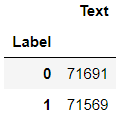
We look at what happened:

 df_train.groupby('Label').count()
      
      

        
        
        
      

    
        
        
        
      
      

        
        
        
      

    
     

 df_val.groupby('Label').count()
      
      

        
        
        
      

    
        
        
        
      
      

        
        
        
      

    
     

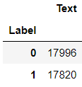
 df_test.groupby('Label').count()
      
      

        
        
        
      

    
        
        
        
      
      

        
        
        
      

    
     

Learning a language model

Loading data:

 tokenizer=Tokenizer(lang='xx') data_lm = TextLMDataBunch.from_df(path, tokenizer=tokenizer, bs=16, train_df=df_train, valid_df=df_val, text_cols=0)
      
      

        
        
        
      

    
        
        
        
      
      

        
        
        
      

    
     

We look at the contents:

 data_lm.show_batch()
      
      

        
        
        
      

    
        
        
        
      
      

        
        
        
      

    
     

We provide links to the stored weights of the pre - trained model and a dictionary:

 weights_pretrained = 'ULMFit/lm_5_ep_lr2-3_5_stlr' itos_pretrained = 'ULMFit/itos' pretained_data = (weights_pretrained, itos_pretrained)
      
      

        
        
        
      

    
        
        
        
      
      

        
        
        
      

    
     

We create learner, but before that - one crutch for fast.ai. The pre-trained model was trained on an older version of the library, so you need to adjust the number of nodes in the hidden layer of the neural network.

 config = awd_lstm_lm_config.copy() config['n_hid'] = 1150 learn_lm = language_model_learner(data_lm, AWD_LSTM, config=config, pretrained_fnames=pretained_data, drop_mult=0.3) learn_lm.freeze()
      
      

        
        
        
      

    
        
        
        
      
      

        
        
        
      

    
     

We are looking for the optimal learning rate:

 learn_lm.lr_find() learn_lm.recorder.plot()
      
      

        
        
        
      

    
        
        
        
      
      

        
        
        
      

    
     

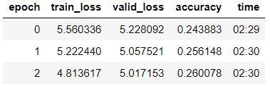
We train the model of the 3rd era (in the model only the last group of layers is unfrozen)

 learn_lm.fit_one_cycle(3, 1e-2, moms=(0.8, 0.7))
      
      

        
        
        
      

    
        
        
        
      
      

        
        
        
      

    
     

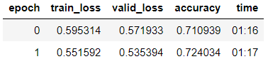
Defrosting the model, teaching 5 more eras with a lower learning rate:

 learn_lm.unfreeze() learn_lm.fit_one_cycle(5, 1e-3, moms=(0.8, 0.7))
      
      

        
        
        
      

    
        
        
        
      
      

        
        
        
      

    
     

 learn_lm.save('lm_ft')
      
      

        
        
        
      

    
        
        
        
      
      

        
        
        
      

    
     

We are trying to generate text on a trained model.

 learn_lm.predict("  ", n_words=5)
      
      

        
        
        
      

    
        
        
        
      
      

        
        
        
      

    
     

 Out: '       '
      
      

        
        
        
      

    
        
        
        
      
      

        
        
        
      

    
     

 learn_lm.predict(",  ", n_words=4)
      
      

        
        
        
      

    
        
        
        
      
      

        
        
        
      

    
     

 Out: ',      '
      
      

        
        
        
      

    
        
        
        
      
      

        
        
        
      

    
     

We see - something that the model does. But our main task is classification, and for its solution we will take an encoder from the model.

 learn_lm.save_encoder('ft_enc')
      
      

        
        
        
      

    
        
        
        
      
      

        
        
        
      

    
     

We train the classifier

Download data for training

 data_clas = TextClasDataBunch.from_df(path, vocab=data_lm.train_ds.vocab, bs=32, train_df=df_train, valid_df=df_val, text_cols=0, label_cols=1, tokenizer=tokenizer)
      
      

        
        
        
      

    
        
        
        
      
      

        
        
        
      

    
     

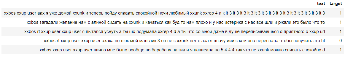
Let's look at the data, we see that the labels were successfully counted (0 means negative, and 1 means a positive comment):

 data_clas.show_batch()
      
      

        
        
        
      

    
        
        
        
      
      

        
        
        
      

    
     

Create a learner with a similar crutch:

 config = awd_lstm_clas_config.copy() config['n_hid'] = 1150 learn = text_classifier_learner(data_clas, AWD_LSTM, config=config, drop_mult=0.5)
      
      

        
        
        
      

    
        
        
        
      
      

        
        
        
      

    
     

We load the encoder trained in the previous step and freeze the model, except for the last group of weights:

 learn.load_encoder('ft_enc') learn.freeze()
      
      

        
        
        
      

    
        
        
        
      
      

        
        
        
      

    
     

We are looking for the optimal learning rate:

 learn.lr_find() learn.recorder.plot(skip_start=0)
      
      

        
        
        
      

    
        
        
        
      
      

        
        
        
      

    
     

We train the model with the gradual thawing of layers.

 learn.fit_one_cycle(2, 2e-2, moms=(0.8,0.7))
      
      

        
        
        
      

    
        
        
        
      
      

        
        
        
      

    
     

 learn.freeze_to(-2) learn.fit_one_cycle(3, slice(1e-2/(2.6**4),1e-2), moms=(0.8,0.7))
      
      

        
        
        
      

    
        
        
        
      
      

        
        
        
      

    
     

 learn.freeze_to(-3) learn.fit_one_cycle(2, slice(5e-3/(2.6**4),5e-3), moms=(0.8,0.7))
      
      

        
        
        
      

    
        
        
        
      
      

        
        
        
      

    
     

 learn.unfreeze() learn.fit_one_cycle(2, slice(1e-3/(2.6**4),1e-3), moms=(0.8,0.7))
      
      

        
        
        
      

    
        
        
        
      
      

        
        
        
      

    
     

 learn.save('tweet-0801')
      
      

        
        
        
      

    
        
        
        
      
      

        
        
        
      

    
     

We see that in the validation sample they achieved accuracy = 80.1%.



We test the model on the ZlodeiBaal comment on my previous article:

 learn.predict('        — ?')
      
      

        
        
        
      

    
        
        
        
      
      

        
        
        
      

    
     

 Out: (Category 0, tensor(0), tensor([0.6283, 0.3717]))
      
      

        
        
        
      

    
        
        
        
      
      

        
        
        
      

    
     

We see that the model attributed this comment to negative :-)

Checking the model on a test sample

The main task at this stage is to test the model for generalization ability. To do this, we validate the model on the dataset stored in the DataFrame df_test, which until then was not available for the language model or for the classifier.

 data_test_clas = TextClasDataBunch.from_df(path, vocab=data_lm.train_ds.vocab, bs=32, train_df=df_train, valid_df=df_test, text_cols=0, label_cols=1, tokenizer=tokenizer)
      
      

        
        
        
      

    
        
        
        
      
      

        
        
        
      

    
     

 config = awd_lstm_clas_config.copy() config['n_hid'] = 1150 learn_test = text_classifier_learner(data_test_clas, AWD_LSTM, config=config, drop_mult=0.5)
      
      

        
        
        
      

    
        
        
        
      
      

        
        
        
      

    
     

 learn_test.load_encoder('ft_enc') learn_test.load('tweet-0801')
      
      

        
        
        
      

    
        
        
        
      
      

        
        
        
      

    
     

 learn_test.validate()
      
      

        
        
        
      

    
        
        
        
      
      

        
        
        
      

    
     

 Out: [0.4391682, tensor(0.7973)]
      
      

        
        
        
      

    
        
        
        
      
      

        
        
        
      

    
     

We see that accuracy on the test sample turned out to be 79.7%.



Let's look at the Confusion Matrix:

 interp = ClassificationInterpretation.from_learner(learn) interp.plot_confusion_matrix()
      
      

        
        
        
      

    
        
        
        
      
      

        
        
        
      

    
     

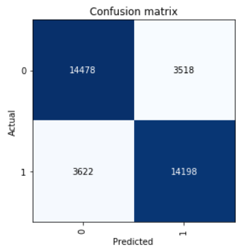
We calculate the precision, recall, and f1 score parameters.

 neg_precision = interp.confusion_matrix()[0][0] / (interp.confusion_matrix()[0][0] + interp.confusion_matrix()[1][0]) neg_recall = interp.confusion_matrix()[0][0] / (interp.confusion_matrix()[0][0] + interp.confusion_matrix()[0][1]) pos_precision = interp.confusion_matrix()[1][1] / (interp.confusion_matrix()[1][1] + interp.confusion_matrix()[0][1]) pos_recall = interp.confusion_matrix()[1][1] / (interp.confusion_matrix()[1][1] + interp.confusion_matrix()[1][0]) neg_f1score = 2 * (neg_precision * neg_recall) / (neg_precision + neg_recall) pos_f1score = 2 * (pos_precision * pos_recall) / (pos_precision + pos_recall)
      
      

        
        
        
      

    
        
        
        
      
      

        
        
        
      

    
     

 print('    F1-score') print(' Negative {0:1.5f} {1:1.5f} {2:1.5f}'.format(neg_precision, neg_recall, neg_f1score)) print(' Positive {0:1.5f} {1:1.5f} {2:1.5f}'.format(pos_precision, pos_recall, pos_f1score)) print(' Average {0:1.5f} {1:1.5f} {2:1.5f}'.format(statistics.mean([neg_precision, pos_precision]), statistics.mean([neg_recall, pos_recall]), statistics.mean([neg_f1score, pos_f1score])))
      
      

        
        
        
      

    
        
        
        
      
      

        
        
        
      

    
     

 Out:     F1-score Negative 0.79989 0.80451 0.80219 Positive 0.80142 0.79675 0.79908 Average 0.80066 0.80063 0.80064
      
      

        
        
        
      

    
        
        
        
      
      

        
        
        
      

    
     

The result shown in the test sample average F1-score = 0.80064.



Saved model weights can be taken here .