A Boring NumPy Tutorial
My name is Vyacheslav, I am a chronic mathematician and for several years I have not used cycles when working with arrays ...
Exactly since I discovered vector operations in NumPy. I want to introduce you to the NumPy functions that I most often use to process arrays of data and images. At the end of the article I will show how you can use the NumPy toolkit to convolve images without iterations (= very fast).
Do not forget about
and let's go!
Content
What is numpy?
Array creation
Access to elements, slices
Array shape and its change
Axis rearrangement and transposition
Array joining
Data cloning
Mathematical operations on array elements
Matrix multiplication
Aggregators
Instead of a conclusion - an example
This is an open source library that once separated from the SciPy project. NumPy is the descendant of Numeric and NumArray. NumPy is based on the LAPAC library, which is written in Fortran. A non-python alternative for NumPy is Matlab.
Due to the fact that NumPy is based on Fortran, it is a fast library. And due to the fact that it supports vector operations with multidimensional arrays, it is extremely convenient.
In addition to the base case (multidimensional arrays in the base case) NumPy includes a set of packages for solving specialized tasks, for example:
So, I propose to consider in detail only a few NumPy features and examples of their use, which will be enough for you to understand how powerful this tool is!
<up>
There are several ways to create an array:
Note that in method No. 3, the dimensions of the array were passed as one parameter (a tuple of sizes). The second parameter in methods No. 3 and No. 4, you can specify the desired type of array elements:
Using the astype method, you can cast the array to a different type. The desired type is indicated as a parameter:
All available types can be found in the sctypes dictionary:
<up>
Access to the elements of the array is carried out by integer indices, the countdown starts from 0:
If you imagine a multidimensional array as a system of nested one-dimensional arrays (a linear array, whose elements can be linear arrays), it becomes obvious that you can access subarrays using an incomplete set of indices:
Given this paradigm, we can rewrite the example of access to one element:
When using an incomplete set of indices, the missing indices are implicitly replaced by a list of all possible indices along the corresponding axis. You can do this explicitly by setting ":". The previous example with one index can be rewritten as follows:
You can “skip” the index along any axis or axes, if the “skipped” axis is followed by axes with indexing, then ":" must:
Indexes can take negative integer values. In this case, the count is from the end of the array:
You can use not single indexes, but lists of indexes along each axis:
Or index ranges in the form “From: To: Step”. This design is called a slice. All elements are selected from the list of indices starting from the From index inclusively, to the To index not including with Step step:
The index step has a default value of 1 and can be skipped:
The From and To values also have default values: 0 and the size of the array along the index axis, respectively:
If you want to use From and To by default (all indices on this axis) and the step is different from 1, then you need to use two pairs of colons so that the interpreter can identify a single parameter as Step. The following code "expands" the array along the second axis, but does not change along the first:
Now let's do it
As you can see, through B we changed the data in A. That's why it is important to use copies in real tasks. The example above should look like this:
NumPy also provides the ability to access multiple array elements through a Boolean indexed array. The index array must match the shape of the indexed one.
As you can see, such a construction returns a flat array consisting of elements of the indexed array that correspond to true indexes. However, if we use such access to the elements of the array to change their values, then the shape of the array will be preserved:
Logical operations logical_and, logical_or, and logical_not are defined over indexing Boolean arrays and perform logical operations AND, OR, and NOT elementwise:
logical_and and logical_or take 2 operands, logical_not take one. You can use the operators &, | and ~ to execute AND, OR, and NOT, respectively, with any number of operands:
Which is equivalent to using only I1.
It is possible to obtain an indexing logical array corresponding in form to an array of values by writing a logical condition with the name of the array as an operand. The boolean value of the index will be calculated as the truth of the expression for the corresponding array element.
Find an indexing array of I elements that are greater than 3, and elements with values less than 2 and more than 4 will be reset to zero:
<up>
A multidimensional array can be represented as a one-dimensional array of maximum length, cut into fragments along the length of the very last axis and laid in layers along the axes, starting with the latter.
For clarity, consider an example:
In this example, we formed 2 new arrays from a one-dimensional array with a length of 24 elements. Array B, size 4 by 6. If you look at the order of values, you can see that along the second dimension there are chains of sequential values.
In array C, 4 by 3 by 2, continuous values run along the last axis. Along the second axis are blocks in series, the combination of which would result in a row along the second axis of array B.
And given that we did not make copies, it becomes clear that these are different forms of representation of the same data array. Therefore, you can easily and quickly change the shape of the array without changing the data itself.
To find out the dimension of the array (number of axes), you can use the ndim field (number), and to find out the size along each axis - shape (tuple). Dimension can also be recognized by the length of the shape. To find out the total number of elements in an array, you can use the size value:
Note that ndim and shape are attributes, not methods!
To see the array one-dimensional, you can use the ravel function:
To resize along the axes or dimension, use the reshape method:
It is important that the number of elements is preserved. Otherwise, an error will occur:
Given that the number of elements is constant, the size along any one axis when performing a reshape can be calculated from the length values along other axes. The size along one axis can be designated -1 and then it will be calculated automatically:
You can use reshape instead of ravel:
Consider the practical application of some of the features for image processing. As the object of study we will use the photo:

Let's try to download and visualize it using Python. For this we need OpenCV and Matplotlib:
The result will be like this:
Pay attention to the download bar:
OpenCV works with images in the BGR format, and we are familiar with RGB. We change the byte order along the color axis without accessing OpenCV functions using the construct
"[:, :, ::-one]".
Reduce the image by 2 times on each axis. Our image has even dimensions along the axes, respectively, can be reduced without interpolation:
Changing the shape of the array, we got 2 new axes, 2 values in each, they correspond to frames composed of odd and even rows and columns of the original image.
Poor quality is due to the use of Matplotlib, because there you can see the dimensions along the axes. In fact, the quality of the thumbnail is:

<up>
In addition to changing the shape of the array with the same order of data units, it is often necessary to change the order of the axes, which will naturally entail permutation of the data blocks.
An example of such a transformation is the transposition of a matrix: interchanging rows and columns.
In this example, the AT construct was used to transpose the matrix A. The transpose operator inverts the axis order. Consider another example with three axes:
This short entry has a longer counterpart: np.transpose (A). This is a more versatile tool for replacing the axis order. The second parameter allows you to specify a tuple of axis numbers of the source array, which determines the order of their position in the resulting array.
For example, rearrange the first two axes of the image. The picture should turn over, but leave the color axis unchanged:
For this example, another swapaxes tool could be used. This method interchanges the two axes specified in the parameters. The example above could be implemented like this:
<up>
Merged arrays must have the same number of axes. Arrays can be combined with the formation of a new axis, or along an existing one.
To combine with the formation of a new axis, the original arrays must have the same dimensions along all axes:
As you can see from the example, the operand arrays became subarrays of the new object and were lined up along the new axis, which is the very first in order.
To combine arrays along an existing axis, they must have the same size on all axes except the one selected for joining, and along it can have arbitrary sizes:
To combine along the first or second axis, you can use the vstack and hstack methods, respectively. We show this with an example of images. vstack combines images of the same width in height, and hsstack combines the same height images in one wide:


Please note that in all examples of this section, the joined arrays are passed by one parameter (tuple). The number of operands can be any, but not necessarily only 2.
Also pay attention to what happens to memory when combining arrays:
Since a new object is created, the data in it is copied from the original arrays, so changes in the new data do not affect the original.
<up>
The np.repeat (A, n) operator will return a one-dimensional array with elements of array A, each of which will be repeated n times.
After this conversion, you can rebuild the geometry of the array and collect duplicate data in one axis:
This option differs from combining the array with the stack operator itself only in the position of the axis along which the same data is placed. In the example above, this is the last axis, if you use stack - the first:
No matter how the data is cloned, the next step is to move the axis along which the same values stand to any position with the axis system:
If we want to “stretch” any axis using the repetition of elements, then the axis with the same values must be put after the expandable (using transpose), and then combine these two axes (using reshape). Consider an example with stretching an image along a vertical axis by duplicating rows:
<up>
If A and B are arrays of the same size, then they can be added, multiplied, subtracted, divided and raised to a power. These operations are performed element by element , the resulting array will coincide in geometry with the original arrays, and each of its elements will be the result of the corresponding operation on a pair of elements from the original arrays:
You can perform any operation from the above on the array and number. In this case, the operation will also be performed on each of the elements of the array:
Considering that a multidimensional array can be considered as a flat array (first axis), whose elements are arrays (other axes), it is possible to perform the considered operations on arrays A and B in the case when the geometry of B coincides with the geometry of the subarrays A at a fixed value along the first axis . In other words, with the same number of axes and sizes A [i] and B. In this case, each of the arrays A [i] and B will be operands for operations defined on arrays.
In this example, array B is subjected to operation with each row of array A. If you need to multiply / divide / add / subtract / raise the degree of subarrays along another axis, you need to use transposition to put the desired axis in its first place, and then return it to its place. Consider the example above, but with multiplication by the vector B of the columns of array A:
For more complex functions (for example, trigonometric, exponent, logarithm, conversion between degrees and radians, module, square root, etc.), there is an implementation in NumPy. Consider the example of exponential and logarithm:
A complete list of mathematical operations in NumPy can be found here .
<up>
The above operation of the product of arrays is performed elementwise. And if you need to perform operations according to the rules of linear algebra over arrays as over tensors, you can use the dot (A, B) method. Depending on the type of operands, the function will perform:
To perform the operations, the corresponding sizes must coincide: for length vectors, for tensors, the lengths along the axes along which the element-wise products will be summed.
Consider examples with scalars and vectors:
With tensors, we will only look at how the geometry of the resulting array changes in size:
To perform a tensor product using other axes, instead of those defined for dot, you can use tensordot with an explicit axis:
We have explicitly indicated that we use the third axis of the first array and the second - of the second (the sizes along these axes must match).
<up>
Aggregators are NumPy methods that allow you to replace data with integral characteristics along some axes. For example, you can calculate the average value, maximum, minimum, variation or some other characteristic along any axis or axes and form a new array from this data. The shape of the new array will contain all the axes of the original array, except those along which the aggregator was counted.
For an example, we will form an array with random values. Then we find the minimum, maximum and average value in its columns:
With this use, mean and average look like synonyms. But these functions have a different set of additional parameters. There are different possibilities for masking and weighting averaged data.
You can calculate the integral characteristics on several axes:
In this example, another integral characteristic sum is considered - the sum.
The list of aggregators looks something like this:
In the case of using argmin and argmax (respectively, both nanargmin and nanargmax), you must specify one axis along which the characteristic will be considered.
If you do not specify an axis, then by default all considered characteristics are considered throughout the array. In this case, argmin and argmax also work correctly and find the index of the maximum or minimum element, as if all the data in the array were stretched along the same axis with the ravel () command.
It should also be noted that aggregation methods are defined not only as methods of the NumPy module, but also for the arrays themselves: the entry np.aggregator (A, axes) is equivalent to the entry A.aggregator (axes), where aggregator means one of the functions considered above, and by axes - axis indices.
<up>
Let's build an algorithm for linear low-pass image filtering.
To get started, upload a noisy image.

Consider a fragment of the image to see the noise:

We will filter the image using a Gaussian filter. But instead of doing the convolution directly (with iteration), we apply the weighted averaging of image slices shifted relative to each other:
We apply this function to our image once, twice and thrice:
We get the following results:


with a single use of the filter;


with double;


at three times.
It can be seen that with an increase in the number of filter passes, the noise level decreases. But this also reduces the clarity of the image. This is a known issue with linear filters. But our image denoising method does not claim to be optimal: this is just a demonstration of the capabilities of NumPy to implement convolution without iterations.
Now let's see the convolution with which kernels our filtering is equivalent. To do this, we will subject a single unit impulse to similar transformations and visualize. In fact, the impulse will not be single, but equal in amplitude to 255, since the mixing itself is optimized for integer data. But this does not interfere with evaluating the general appearance of the nuclei:
We considered a far from complete set of NumPy features, I hope this was enough to demonstrate the full power and beauty of this tool!
<up>
Exactly since I discovered vector operations in NumPy. I want to introduce you to the NumPy functions that I most often use to process arrays of data and images. At the end of the article I will show how you can use the NumPy toolkit to convolve images without iterations (= very fast).
Do not forget about
import numpy as np
and let's go!
Content
What is numpy?
Array creation
Access to elements, slices
Array shape and its change
Axis rearrangement and transposition
Array joining
Data cloning
Mathematical operations on array elements
Matrix multiplication
Aggregators
Instead of a conclusion - an example
What is numpy?
This is an open source library that once separated from the SciPy project. NumPy is the descendant of Numeric and NumArray. NumPy is based on the LAPAC library, which is written in Fortran. A non-python alternative for NumPy is Matlab.
Due to the fact that NumPy is based on Fortran, it is a fast library. And due to the fact that it supports vector operations with multidimensional arrays, it is extremely convenient.
In addition to the base case (multidimensional arrays in the base case) NumPy includes a set of packages for solving specialized tasks, for example:
- numpy.linalg - implements linear algebra operations (a simple multiplication of vectors and matrices is in the basic version);
- numpy.random - implements functions for working with random variables;
- numpy.fft - implements the direct and inverse Fourier transform.
So, I propose to consider in detail only a few NumPy features and examples of their use, which will be enough for you to understand how powerful this tool is!
<up>
Array creation
There are several ways to create an array:
- convert list to array:
A = np.array([[1, 2, 3], [4, 5, 6]]) A Out: array([[1, 2, 3], [4, 5, 6]])
- copy the array (copy and deep copy required !!!):
B = A.copy() B Out: array([[1, 2, 3], [4, 5, 6]])
- create a zero or one array of a given size:
A = np.zeros((2, 3)) A Out: array([[0., 0., 0.], [0., 0., 0.]])
B = np.ones((3, 2)) B Out: array([[1., 1.], [1., 1.], [1., 1.]])
Or take the dimensions of an existing array:
A = np.array([[1, 2, 3], [4, 5, 6]]) B = np.zeros_like(A) B Out: array([[0, 0, 0], [0, 0, 0]])
A = np.array([[1, 2, 3], [4, 5, 6]]) B = np.ones_like(A) B Out: array([[1, 1, 1], [1, 1, 1]])
- when creating a two-dimensional square array, you can make it a unit diagonal matrix:
A = np.eye(3) A Out: array([[1., 0., 0.], [0., 1., 0.], [0., 0., 1.]])
- build an array of numbers from From (including) to To (not including) with Step step:
From = 2.5 To = 7 Step = 0.5 A = np.arange(From, To, Step) A Out: array([2.5, 3. , 3.5, 4. , 4.5, 5. , 5.5, 6. , 6.5])
By default, from = 0, step = 1, therefore, a variant with one parameter is interpreted as To:
A = np.arange(5) A Out: array([0, 1, 2, 3, 4])
Or with two - like From and To:
A = np.arange(10, 15) A Out: array([10, 11, 12, 13, 14])
Note that in method No. 3, the dimensions of the array were passed as one parameter (a tuple of sizes). The second parameter in methods No. 3 and No. 4, you can specify the desired type of array elements:
A = np.zeros((2, 3), 'int') A Out: array([[0, 0, 0], [0, 0, 0]])
B = np.ones((3, 2), 'complex') B Out: array([[1.+0.j, 1.+0.j], [1.+0.j, 1.+0.j], [1.+0.j, 1.+0.j]])
Using the astype method, you can cast the array to a different type. The desired type is indicated as a parameter:
A = np.ones((3, 2)) B = A.astype('str') B Out: array([['1.0', '1.0'], ['1.0', '1.0'], ['1.0', '1.0']], dtype='<U32')
All available types can be found in the sctypes dictionary:
np.sctypes Out: {'int': [numpy.int8, numpy.int16, numpy.int32, numpy.int64], 'uint': [numpy.uint8, numpy.uint16, numpy.uint32, numpy.uint64], 'float': [numpy.float16, numpy.float32, numpy.float64, numpy.float128], 'complex': [numpy.complex64, numpy.complex128, numpy.complex256], 'others': [bool, object, bytes, str, numpy.void]}
<up>
Access to elements, slices
Access to the elements of the array is carried out by integer indices, the countdown starts from 0:
A = np.array([[1, 2, 3], [4, 5, 6]]) A[1, 1] Out: 5
If you imagine a multidimensional array as a system of nested one-dimensional arrays (a linear array, whose elements can be linear arrays), it becomes obvious that you can access subarrays using an incomplete set of indices:
A = np.array([[1, 2, 3], [4, 5, 6]]) A[1] Out: array([4, 5, 6])
Given this paradigm, we can rewrite the example of access to one element:
A = np.array([[1, 2, 3], [4, 5, 6]]) A[1][1] Out: 5
When using an incomplete set of indices, the missing indices are implicitly replaced by a list of all possible indices along the corresponding axis. You can do this explicitly by setting ":". The previous example with one index can be rewritten as follows:
A = np.array([[1, 2, 3], [4, 5, 6]]) A[1, :] Out: array([4, 5, 6])
You can “skip” the index along any axis or axes, if the “skipped” axis is followed by axes with indexing, then ":" must:
A = np.array([[1, 2, 3], [4, 5, 6]]) A[:, 1] Out: array([2, 5])
Indexes can take negative integer values. In this case, the count is from the end of the array:
A = np.arange(5) print(A) A[-1] Out: [0 1 2 3 4] 4
You can use not single indexes, but lists of indexes along each axis:
A = np.arange(5) print(A) A[[0, 1, -1]] Out: [0 1 2 3 4] array([0, 1, 4])
Or index ranges in the form “From: To: Step”. This design is called a slice. All elements are selected from the list of indices starting from the From index inclusively, to the To index not including with Step step:
A = np.arange(5) print(A) A[0:4:2] Out: [0 1 2 3 4] array([0, 2])
The index step has a default value of 1 and can be skipped:
A = np.arange(5) print(A) A[0:4] Out: [0 1 2 3 4] array([0, 1, 2, 3])
The From and To values also have default values: 0 and the size of the array along the index axis, respectively:
A = np.arange(5) print(A) A[:4] Out: [0 1 2 3 4] array([0, 1, 2, 3])
A = np.arange(5) print(A) A[-3:] Out: [0 1 2 3 4] array([2, 3, 4])
If you want to use From and To by default (all indices on this axis) and the step is different from 1, then you need to use two pairs of colons so that the interpreter can identify a single parameter as Step. The following code "expands" the array along the second axis, but does not change along the first:
A = np.array([[1, 2, 3], [4, 5, 6]]) B = A[:, ::-1] print("A", A) print("B", B) Out: A [[1 2 3] [4 5 6]] B [[3 2 1] [6 5 4]]
Now let's do it
print(A) B[0, 0] = 0 print(A) Out: [[1 2 3] [4 5 6]] [[1 2 0] [4 5 6]]
As you can see, through B we changed the data in A. That's why it is important to use copies in real tasks. The example above should look like this:
A = np.array([[1, 2, 3], [4, 5, 6]]) B = A.copy()[:, ::-1] print("A", A) print("B", B) Out: A [[1 2 3] [4 5 6]] B [[3 2 1] [6 5 4]]
NumPy also provides the ability to access multiple array elements through a Boolean indexed array. The index array must match the shape of the indexed one.
A = np.array([[1, 2, 3], [4, 5, 6]]) I = np.array([[False, False, True], [ True, False, True]]) A[I] Out: array([3, 4, 6])
As you can see, such a construction returns a flat array consisting of elements of the indexed array that correspond to true indexes. However, if we use such access to the elements of the array to change their values, then the shape of the array will be preserved:
A = np.array([[1, 2, 3], [4, 5, 6]]) I = np.array([[False, False, True], [ True, False, True]]) A[I] = 0 print(A) Out: [[1 2 0] [0 5 0]]
Logical operations logical_and, logical_or, and logical_not are defined over indexing Boolean arrays and perform logical operations AND, OR, and NOT elementwise:
A = np.array([[1, 2, 3], [4, 5, 6]]) I1 = np.array([[False, False, True], [True, False, True]]) I2 = np.array([[False, True, False], [False, False, True]]) B = A.copy() C = A.copy() D = A.copy() B[np.logical_and(I1, I2)] = 0 C[np.logical_or(I1, I2)] = 0 D[np.logical_not(I1)] = 0 print('B\n', B) print('\nC\n', C) print('\nD\n', D) Out: B [[1 2 3] [4 5 0]] C [[1 0 0] [0 5 0]] D [[0 0 3] [4 0 6]]
logical_and and logical_or take 2 operands, logical_not take one. You can use the operators &, | and ~ to execute AND, OR, and NOT, respectively, with any number of operands:
A = np.array([[1, 2, 3], [4, 5, 6]]) I1 = np.array([[False, False, True], [True, False, True]]) I2 = np.array([[False, True, False], [False, False, True]]) A[I1 & (I1 | ~ I2)] = 0 print(A) Out: [[1 2 0] [0 5 0]]
Which is equivalent to using only I1.
It is possible to obtain an indexing logical array corresponding in form to an array of values by writing a logical condition with the name of the array as an operand. The boolean value of the index will be calculated as the truth of the expression for the corresponding array element.
Find an indexing array of I elements that are greater than 3, and elements with values less than 2 and more than 4 will be reset to zero:
A = np.array([[1, 2, 3], [4, 5, 6]]) print('A before\n', A) I = A > 3 print('I\n', I) A[np.logical_or(A < 2, A > 4)] = 0 print('A after\n', A) Out: A before [[1 2 3] [4 5 6]] I [[False False False] [ True True True]] A after [[0 2 3] [4 0 0]]
<up>
Array shape and its change
A multidimensional array can be represented as a one-dimensional array of maximum length, cut into fragments along the length of the very last axis and laid in layers along the axes, starting with the latter.
For clarity, consider an example:
A = np.arange(24) B = A.reshape(4, 6) C = A.reshape(4, 3, 2) print('B\n', B) print('\nC\n', C) Out: B [[ 0 1 2 3 4 5] [ 6 7 8 9 10 11] [12 13 14 15 16 17] [18 19 20 21 22 23]] C [[[ 0 1] [ 2 3] [ 4 5]] [[ 6 7] [ 8 9] [10 11]] [[12 13] [14 15] [16 17]] [[18 19] [20 21] [22 23]]]
In this example, we formed 2 new arrays from a one-dimensional array with a length of 24 elements. Array B, size 4 by 6. If you look at the order of values, you can see that along the second dimension there are chains of sequential values.
In array C, 4 by 3 by 2, continuous values run along the last axis. Along the second axis are blocks in series, the combination of which would result in a row along the second axis of array B.
And given that we did not make copies, it becomes clear that these are different forms of representation of the same data array. Therefore, you can easily and quickly change the shape of the array without changing the data itself.
To find out the dimension of the array (number of axes), you can use the ndim field (number), and to find out the size along each axis - shape (tuple). Dimension can also be recognized by the length of the shape. To find out the total number of elements in an array, you can use the size value:
A = np.arange(24) C = A.reshape(4, 3, 2) print(C.ndim, C.shape, len(C.shape), A.size) Out: 3 (4, 3, 2) 3 24
Note that ndim and shape are attributes, not methods!
To see the array one-dimensional, you can use the ravel function:
A = np.array([[1, 2, 3], [4, 5, 6]]) A.ravel() Out: array([1, 2, 3, 4, 5, 6])
To resize along the axes or dimension, use the reshape method:
A = np.array([[1, 2, 3], [4, 5, 6]]) A.reshape(3, 2) Out: array([[1, 2], [3, 4], [5, 6]])
It is important that the number of elements is preserved. Otherwise, an error will occur:
A = np.array([[1, 2, 3], [4, 5, 6]]) A.reshape(3, 3) Out: ValueError Traceback (most recent call last) <ipython-input-73-d204e18427d9> in <module> 1 A = np.array([[1, 2, 3], [4, 5, 6]]) ----> 2 A.reshape(3, 3) ValueError: cannot reshape array of size 6 into shape (3,3)
Given that the number of elements is constant, the size along any one axis when performing a reshape can be calculated from the length values along other axes. The size along one axis can be designated -1 and then it will be calculated automatically:
A = np.arange(24) B = A.reshape(4, -1) C = A.reshape(4, -1, 2) print(B.shape, C.shape) Out: (4, 6) (4, 3, 2)
You can use reshape instead of ravel:
A = np.array([[1, 2, 3], [4, 5, 6]]) B = A.reshape(-1) print(B.shape) Out: (6,)
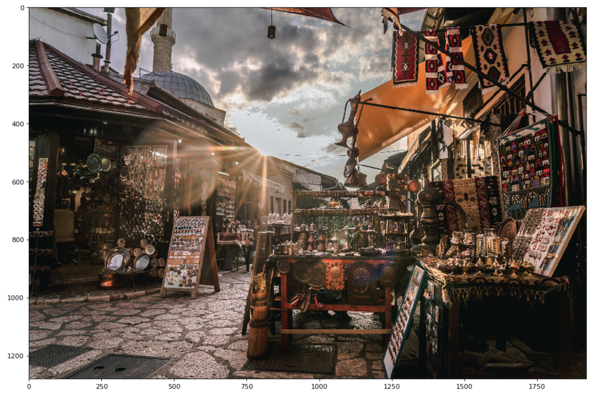
Consider the practical application of some of the features for image processing. As the object of study we will use the photo:
Let's try to download and visualize it using Python. For this we need OpenCV and Matplotlib:
import cv2 from matplotlib import pyplot as plt I = cv2.imread('sarajevo.jpg')[:, :, ::-1] plt.figure(num=None, figsize=(15, 15), dpi=80, facecolor='w', edgecolor='k') plt.imshow(I) plt.show()
The result will be like this:
Pay attention to the download bar:
I = cv2.imread('sarajevo.jpg')[:, :, ::-1] print(I.shape) Out: (1280, 1920, 3)
OpenCV works with images in the BGR format, and we are familiar with RGB. We change the byte order along the color axis without accessing OpenCV functions using the construct
"[:, :, ::-one]".
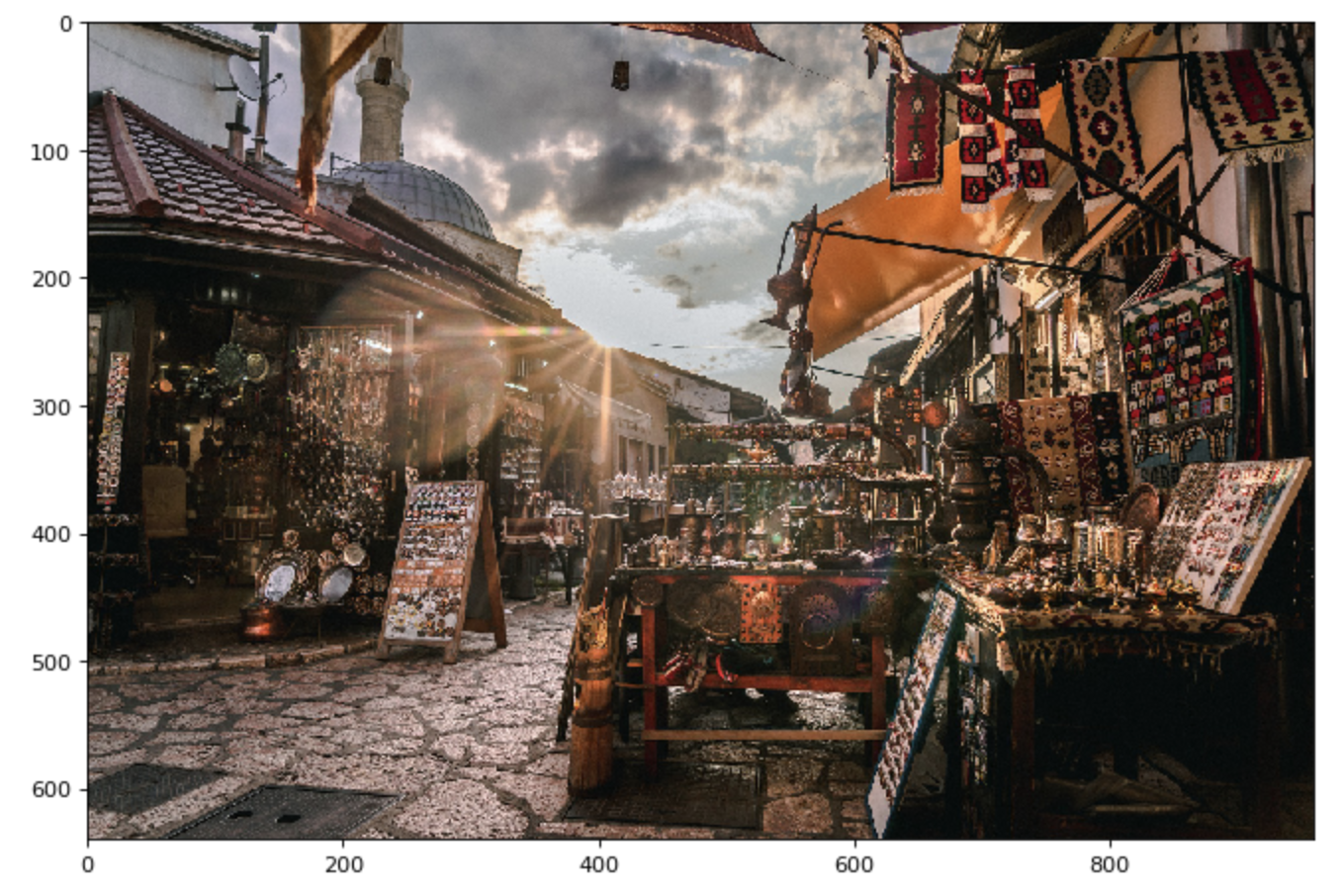
Reduce the image by 2 times on each axis. Our image has even dimensions along the axes, respectively, can be reduced without interpolation:
I_ = I.reshape(I.shape[0] // 2, 2, I.shape[1] // 2, 2, -1) print(I_.shape) plt.figure(num=None, figsize=(10, 10), dpi=80, facecolor='w', edgecolor='k') plt.imshow(I_[:, 0, :, 0]) plt.show()
Changing the shape of the array, we got 2 new axes, 2 values in each, they correspond to frames composed of odd and even rows and columns of the original image.
Poor quality is due to the use of Matplotlib, because there you can see the dimensions along the axes. In fact, the quality of the thumbnail is:
<up>
Axis rearrangement and transposition
In addition to changing the shape of the array with the same order of data units, it is often necessary to change the order of the axes, which will naturally entail permutation of the data blocks.
An example of such a transformation is the transposition of a matrix: interchanging rows and columns.
A = np.array([[1, 2, 3], [4, 5, 6]]) print('A\n', A) print('\nA data\n', A.ravel()) B = AT print('\nB\n', B) print('\nB data\n', B.ravel()) Out: A [[1 2 3] [4 5 6]] A data [1 2 3 4 5 6] B [[1 4] [2 5] [3 6]] B data [1 4 2 5 3 6]
In this example, the AT construct was used to transpose the matrix A. The transpose operator inverts the axis order. Consider another example with three axes:
C = np.arange(24).reshape(4, -1, 2) print(C.shape, np.transpose(C).shape) print() print(C[0]) print() print(CT[:, :, 0]) Out: [[0 1] [2 3] [4 5]] [[0 2 4] [1 3 5]]
This short entry has a longer counterpart: np.transpose (A). This is a more versatile tool for replacing the axis order. The second parameter allows you to specify a tuple of axis numbers of the source array, which determines the order of their position in the resulting array.
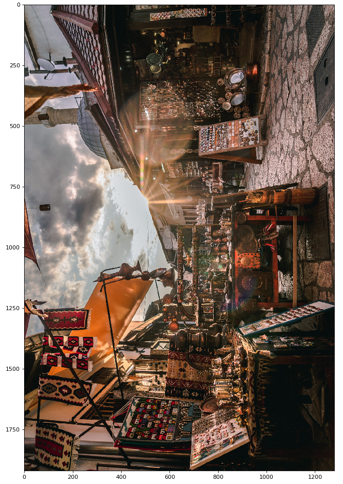
For example, rearrange the first two axes of the image. The picture should turn over, but leave the color axis unchanged:
I_ = np.transpose(I, (1, 0, 2)) plt.figure(num=None, figsize=(15, 15), dpi=80, facecolor='w', edgecolor='k') plt.imshow(I_) plt.show()
For this example, another swapaxes tool could be used. This method interchanges the two axes specified in the parameters. The example above could be implemented like this:
I_ = np.swapaxes(I, 0, 1)
<up>
Array joining
Merged arrays must have the same number of axes. Arrays can be combined with the formation of a new axis, or along an existing one.
To combine with the formation of a new axis, the original arrays must have the same dimensions along all axes:
A = np.array([[1, 2, 3, 4], [5, 6, 7, 8]]) B = A[::-1] C = A[:, ::-1] D = np.stack((A, B, C)) print(D.shape) D Out: (3, 2, 4) array([[[1, 2, 3, 4], [5, 6, 7, 8]], [[5, 6, 7, 8], [1, 2, 3, 4]], [[4, 3, 2, 1], [8, 7, 6, 5]]])
As you can see from the example, the operand arrays became subarrays of the new object and were lined up along the new axis, which is the very first in order.
To combine arrays along an existing axis, they must have the same size on all axes except the one selected for joining, and along it can have arbitrary sizes:
A = np.ones((2, 1, 2)) B = np.zeros((2, 3, 2)) C = np.concatenate((A, B), 1) print(C.shape) C Out: (2, 4, 2) array([[[1., 1.], [0., 0.], [0., 0.], [0., 0.]], [[1., 1.], [0., 0.], [0., 0.], [0., 0.]]])
To combine along the first or second axis, you can use the vstack and hstack methods, respectively. We show this with an example of images. vstack combines images of the same width in height, and hsstack combines the same height images in one wide:
I = cv2.imread('sarajevo.jpg')[:, :, ::-1] I_ = I.reshape(I.shape[0] // 2, 2, I.shape[1] // 2, 2, -1) Ih = np.hstack((I_[:, 0, :, 0], I_[:, 0, :, 1])) Iv = np.vstack((I_[:, 0, :, 0], I_[:, 1, :, 0])) plt.figure(num=None, figsize=(10, 10), dpi=80, facecolor='w', edgecolor='k') plt.imshow(Ih) plt.show() plt.figure(num=None, figsize=(10, 10), dpi=80, facecolor='w', edgecolor='k') plt.imshow(Iv) plt.show()
Please note that in all examples of this section, the joined arrays are passed by one parameter (tuple). The number of operands can be any, but not necessarily only 2.
Also pay attention to what happens to memory when combining arrays:
A = np.array([[1, 2, 3, 4], [5, 6, 7, 8]]) B = A[::-1] C = A[:, ::-1] D = np.stack((A, B, C)) D[0, 0, 0] = 0 print(A) Out: [[1 2 3 4] [5 6 7 8]]
Since a new object is created, the data in it is copied from the original arrays, so changes in the new data do not affect the original.
<up>
Data cloning
The np.repeat (A, n) operator will return a one-dimensional array with elements of array A, each of which will be repeated n times.
A = np.array([[1, 2, 3, 4], [5, 6, 7, 8]]) print(np.repeat(A, 2)) Out: [1 1 2 2 3 3 4 4 5 5 6 6 7 7 8 8]
After this conversion, you can rebuild the geometry of the array and collect duplicate data in one axis:
A = np.array([[1, 2, 3, 4], [5, 6, 7, 8]]) B = np.repeat(A, 2).reshape(A.shape[0], A.shape[1], -1) print(B) Out: [[[1 1] [2 2] [3 3] [4 4]] [[5 5] [6 6] [7 7] [8 8]]]
This option differs from combining the array with the stack operator itself only in the position of the axis along which the same data is placed. In the example above, this is the last axis, if you use stack - the first:
A = np.array([[1, 2, 3, 4], [5, 6, 7, 8]]) B = np.stack((A, A)) print(B) Out: [[[1 2 3 4] [5 6 7 8]] [[1 2 3 4] [5 6 7 8]]]
No matter how the data is cloned, the next step is to move the axis along which the same values stand to any position with the axis system:
A = np.array([[1, 2, 3, 4], [5, 6, 7, 8]]) B = np.transpose(np.stack((A, A)), (1, 0, 2)) C = np.transpose(np.repeat(A, 2).reshape(A.shape[0], A.shape[1], -1), (0, 2, 1)) print('B\n', B) print('\nC\n', C) Out: B [[[1 2 3 4] [1 2 3 4]] [[5 6 7 8] [5 6 7 8]]] C [[[1 2 3 4] [1 2 3 4]] [[5 6 7 8] [5 6 7 8]]]
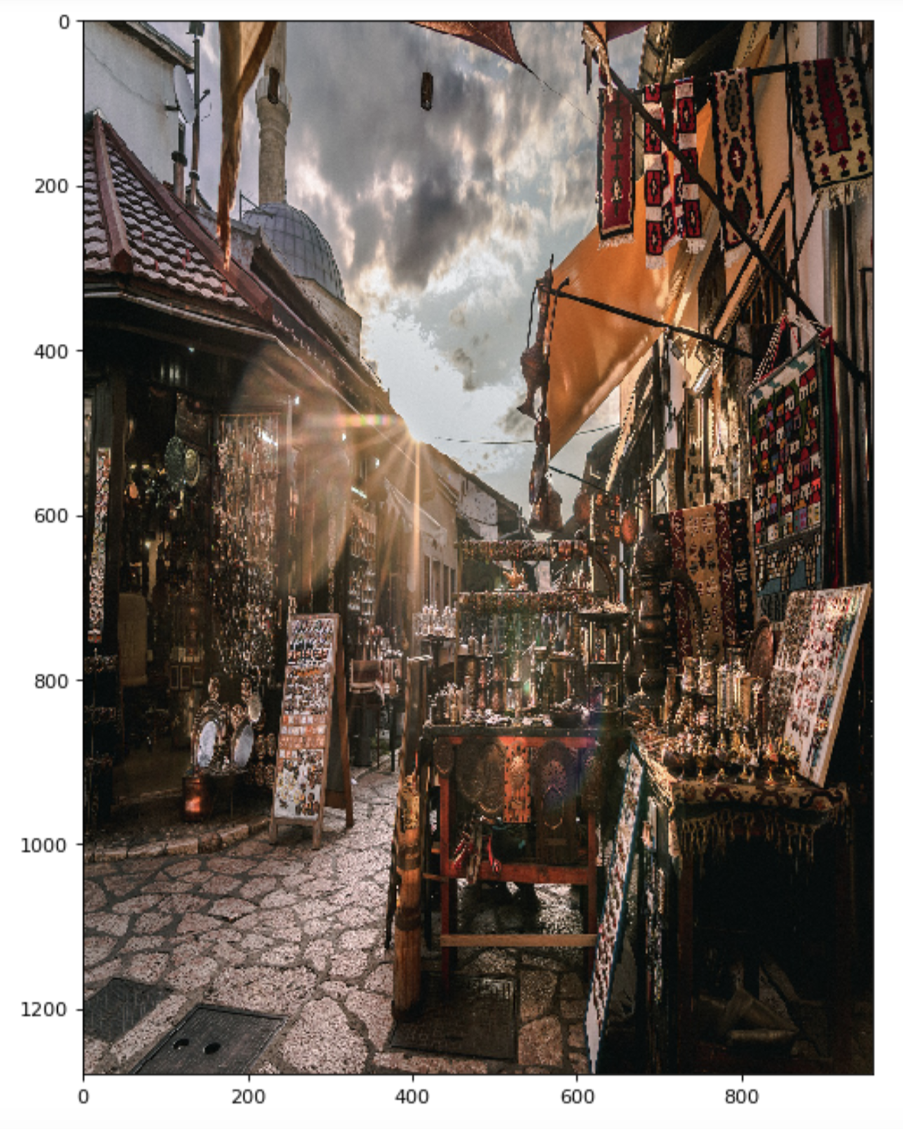
If we want to “stretch” any axis using the repetition of elements, then the axis with the same values must be put after the expandable (using transpose), and then combine these two axes (using reshape). Consider an example with stretching an image along a vertical axis by duplicating rows:
I0 = cv2.imread('sarajevo.jpg')[:, :, ::-1] # I1 = I.reshape(I.shape[0] // 2, 2, I.shape[1] // 2, 2, -1)[:, 0, :, 0] # I2 = np.repeat(I1, 2) # I3 = I2.reshape(I1.shape[0], I1.shape[1], I1.shape[2], -1) I4 = np.transpose(I3, (0, 3, 1, 2)) # I5 = I4.reshape(-1, I1.shape[1], I1.shape[2]) # print('I0', I0.shape) print('I1', I1.shape) print('I2', I2.shape) print('I3', I3.shape) print('I4', I4.shape) print('I5', I5.shape) plt.figure(num=None, figsize=(10, 10), dpi=80, facecolor='w', edgecolor='k') plt.imshow(I5) plt.show() Out: I0 (1280, 1920, 3) I1 (640, 960, 3) I2 (3686400,) I3 (640, 960, 3, 2) I4 (640, 2, 960, 3) I5 (1280, 960, 3)
<up>
Mathematical operations on array elements
If A and B are arrays of the same size, then they can be added, multiplied, subtracted, divided and raised to a power. These operations are performed element by element , the resulting array will coincide in geometry with the original arrays, and each of its elements will be the result of the corresponding operation on a pair of elements from the original arrays:
A = np.array([[-1., 2., 3.], [4., 5., 6.], [7., 8., 9.]]) B = np.array([[1., -2., -3.], [7., 8., 9.], [4., 5., 6.], ]) C = A + B D = A - B E = A * B F = A / B G = A ** B print('+\n', C, '\n') print('-\n', D, '\n') print('*\n', E, '\n') print('/\n', F, '\n') print('**\n', G, '\n') Out: + [[ 0. 0. 0.] [11. 13. 15.] [11. 13. 15.]] - [[-2. 4. 6.] [-3. -3. -3.] [ 3. 3. 3.]] * [[-1. -4. -9.] [28. 40. 54.] [28. 40. 54.]] / [[-1. -1. -1. ] [ 0.57142857 0.625 0.66666667] [ 1.75 1.6 1.5 ]] ** [[-1.0000000e+00 2.5000000e-01 3.7037037e-02] [ 1.6384000e+04 3.9062500e+05 1.0077696e+07] [ 2.4010000e+03 3.2768000e+04 5.3144100e+05]]
You can perform any operation from the above on the array and number. In this case, the operation will also be performed on each of the elements of the array:
A = np.array([[-1., 2., 3.], [4., 5., 6.], [7., 8., 9.]]) B = -2. C = A + B D = A - B E = A * B F = A / B G = A ** B print('+\n', C, '\n') print('-\n', D, '\n') print('*\n', E, '\n') print('/\n', F, '\n') print('**\n', G, '\n') Out: + [[-3. 0. 1.] [ 2. 3. 4.] [ 5. 6. 7.]] - [[ 1. 4. 5.] [ 6. 7. 8.] [ 9. 10. 11.]] * [[ 2. -4. -6.] [ -8. -10. -12.] [-14. -16. -18.]] / [[ 0.5 -1. -1.5] [-2. -2.5 -3. ] [-3.5 -4. -4.5]] ** [[1. 0.25 0.11111111] [0.0625 0.04 0.02777778] [0.02040816 0.015625 0.01234568]]
Considering that a multidimensional array can be considered as a flat array (first axis), whose elements are arrays (other axes), it is possible to perform the considered operations on arrays A and B in the case when the geometry of B coincides with the geometry of the subarrays A at a fixed value along the first axis . In other words, with the same number of axes and sizes A [i] and B. In this case, each of the arrays A [i] and B will be operands for operations defined on arrays.
A = np.array([[1., 2., 3.], [4., 5., 6.], [7., 8., 9.]]) B = np.array([-1.1, -1.2, -1.3]) C = AT + B D = AT - B E = AT * B F = AT / B G = AT ** B print('+\n', C, '\n') print('-\n', D, '\n') print('*\n', E, '\n') print('/\n', F, '\n') print('**\n', G, '\n') Out: + [[-0.1 2.8 5.7] [ 0.9 3.8 6.7] [ 1.9 4.8 7.7]] - [[ 2.1 5.2 8.3] [ 3.1 6.2 9.3] [ 4.1 7.2 10.3]] * [[ -1.1 -4.8 -9.1] [ -2.2 -6. -10.4] [ -3.3 -7.2 -11.7]] / [[-0.90909091 -3.33333333 -5.38461538] [-1.81818182 -4.16666667 -6.15384615] [-2.72727273 -5. -6.92307692]] ** [[1. 0.18946457 0.07968426] [0.4665165 0.14495593 0.06698584] [0.29865282 0.11647119 0.05747576]]
In this example, array B is subjected to operation with each row of array A. If you need to multiply / divide / add / subtract / raise the degree of subarrays along another axis, you need to use transposition to put the desired axis in its first place, and then return it to its place. Consider the example above, but with multiplication by the vector B of the columns of array A:
A = np.array([[1., 2., 3.], [4., 5., 6.], [7., 8., 9.]]) B = np.array([-1.1, -1.2, -1.3]) C = (AT + B).T D = (AT - B).T E = (AT * B).T F = (AT / B).T G = (AT ** B).T print('+\n', C, '\n') print('-\n', D, '\n') print('*\n', E, '\n') print('/\n', F, '\n') print('**\n', G, '\n') Out: + [[-0.1 0.9 1.9] [ 2.8 3.8 4.8] [ 5.7 6.7 7.7]] - [[ 2.1 3.1 4.1] [ 5.2 6.2 7.2] [ 8.3 9.3 10.3]] * [[ -1.1 -2.2 -3.3] [ -4.8 -6. -7.2] [ -9.1 -10.4 -11.7]] / [[-0.90909091 -1.81818182 -2.72727273] [-3.33333333 -4.16666667 -5. ] [-5.38461538 -6.15384615 -6.92307692]] ** [[1. 0.4665165 0.29865282] [0.18946457 0.14495593 0.11647119] [0.07968426 0.06698584 0.05747576]]
For more complex functions (for example, trigonometric, exponent, logarithm, conversion between degrees and radians, module, square root, etc.), there is an implementation in NumPy. Consider the example of exponential and logarithm:
A = np.array([[1., 2., 3.], [4., 5., 6.], [7., 8., 9.]]) B = np.exp(A) C = np.log(B) print('A', A, '\n') print('B', B, '\n') print('C', C, '\n') Out: A [[1. 2. 3.] [4. 5. 6.] [7. 8. 9.]] B [[2.71828183e+00 7.38905610e+00 2.00855369e+01] [5.45981500e+01 1.48413159e+02 4.03428793e+02] [1.09663316e+03 2.98095799e+03 8.10308393e+03]] C [[1. 2. 3.] [4. 5. 6.] [7. 8. 9.]]
A complete list of mathematical operations in NumPy can be found here .
<up>
Matrix multiplication
The above operation of the product of arrays is performed elementwise. And if you need to perform operations according to the rules of linear algebra over arrays as over tensors, you can use the dot (A, B) method. Depending on the type of operands, the function will perform:
- if the arguments are scalars (numbers), then multiplication will be performed;
- if the arguments are a vector (a one-dimensional array) and a scalar, then the array will be multiplied by a number;
- if the arguments are vector, then scalar multiplication will be performed (the sum of the element-wise products);
- if the arguments are tensor (multidimensional array) and scalar, then the vector will be multiplied by a number;
- if the arguments of the tensor, then the product of the tensors along the last axis of the first argument and the penultimate – second will be executed;
- if the arguments are matrices, then the product of the matrices is executed (this is a special case of the product of tensors);
- if the arguments are matrix and vector, then the product of the matrix and the vector will be executed (this is also a special case of the product of tensors).
To perform the operations, the corresponding sizes must coincide: for length vectors, for tensors, the lengths along the axes along which the element-wise products will be summed.
Consider examples with scalars and vectors:
# A = 2 B = 3 print(np.dot(A, B), '\n') # A = np.array([2., 3., 4.]) B = 3 print(np.dot(A, B), '\n') # A = np.array([2., 3., 4.]) B = np.array([-2., 1., -1.]) print(np.dot(A, B), '\n') # A = np.array([[2., 3., 4.], [5., 6., 7.]]) B = 2 print(np.dot(A, B), '\n') Out: 6 [ 6. 9. 12.] -5.0 [[ 4. 6. 8.] [10. 12. 14.]]
With tensors, we will only look at how the geometry of the resulting array changes in size:
# ( 2) ( 1) A = np.ones((5, 6)) B = np.ones(6) print('A:', A.shape, '\nB:', B.shape, '\nresult:', np.dot(A, B).shape, '\n\n') # ( 2) A = np.ones((5, 6)) B = np.ones((6, 7)) print('A:', A.shape, '\nB:', B.shape, '\nresult:', np.dot(A, B).shape, '\n\n') # A = np.ones((5, 6, 7, 8)) B = np.ones((1, 2, 3, 8, 4)) print('A:', A.shape, '\nB:', B.shape, '\nresult:', np.dot(A, B).shape, '\n\n') Out: A: (5, 6) B: (6,) result: (5,) A: (5, 6) B: (6, 7) result: (5, 7) A: (5, 6, 7, 8) B: (1, 2, 3, 8, 4) result: (5, 6, 7, 1, 2, 3, 4)
To perform a tensor product using other axes, instead of those defined for dot, you can use tensordot with an explicit axis:
A = np.ones((1, 3, 7, 4)) B = np.ones((5, 7, 6, 7, 8)) print('A:', A.shape, '\nB:', B.shape, '\nresult:', np.tensordot(A, B, [2, 1]).shape, '\n\n') Out: A: (1, 3, 7, 4) B: (5, 7, 6, 7, 8) result: (1, 3, 4, 5, 6, 7, 8)
We have explicitly indicated that we use the third axis of the first array and the second - of the second (the sizes along these axes must match).
<up>
Aggregators
Aggregators are NumPy methods that allow you to replace data with integral characteristics along some axes. For example, you can calculate the average value, maximum, minimum, variation or some other characteristic along any axis or axes and form a new array from this data. The shape of the new array will contain all the axes of the original array, except those along which the aggregator was counted.
For an example, we will form an array with random values. Then we find the minimum, maximum and average value in its columns:
A = np.random.rand(4, 5) print('A\n', A, '\n') print('min\n', np.min(A, 0), '\n') print('max\n', np.max(A, 0), '\n') print('mean\n', np.mean(A, 0), '\n') print('average\n', np.average(A, 0), '\n') Out: A [[0.58481838 0.32381665 0.53849901 0.32401355 0.05442121] [0.34301843 0.38620863 0.52689694 0.93233065 0.73474868] [0.09888225 0.03710514 0.17910721 0.05245685 0.00962319] [0.74758173 0.73529492 0.58517879 0.11785686 0.81204847]] min [0.09888225 0.03710514 0.17910721 0.05245685 0.00962319] max [0.74758173 0.73529492 0.58517879 0.93233065 0.81204847] mean [0.4435752 0.37060634 0.45742049 0.35666448 0.40271039] average [0.4435752 0.37060634 0.45742049 0.35666448 0.40271039]
With this use, mean and average look like synonyms. But these functions have a different set of additional parameters. There are different possibilities for masking and weighting averaged data.
You can calculate the integral characteristics on several axes:
A = np.ones((10, 4, 5)) print('sum\n', np.sum(A, (0, 2)), '\n') print('min\n', np.min(A, (0, 2)), '\n') print('max\n', np.max(A, (0, 2)), '\n') print('mean\n', np.mean(A, (0, 2)), '\n') Out: sum [50. 50. 50. 50.] min [1. 1. 1. 1.] max [1. 1. 1. 1.] mean [1. 1. 1. 1.]
In this example, another integral characteristic sum is considered - the sum.
The list of aggregators looks something like this:
- sum: sum and nansum - a variant correctly managing with nan;
- work: prod and nanprod;
- average and expectation: average and mean (nanmean),
there isnonanaverage; - median: median and nanmedian;
- percentile: percentile and nanpercentile;
- variation: var and nanvar;
- standard deviation (square root of variation): std and nanstd;
- : min nanmin;
- : max nanmax;
- , : argmin nanargmin;
- , : argmax nanargmax.
In the case of using argmin and argmax (respectively, both nanargmin and nanargmax), you must specify one axis along which the characteristic will be considered.
If you do not specify an axis, then by default all considered characteristics are considered throughout the array. In this case, argmin and argmax also work correctly and find the index of the maximum or minimum element, as if all the data in the array were stretched along the same axis with the ravel () command.
It should also be noted that aggregation methods are defined not only as methods of the NumPy module, but also for the arrays themselves: the entry np.aggregator (A, axes) is equivalent to the entry A.aggregator (axes), where aggregator means one of the functions considered above, and by axes - axis indices.
A = np.ones((10, 4, 5)) print('sum\n', A.sum((0, 2)), '\n') print('min\n', A.min((0, 2)), '\n') print('max\n', A.max((0, 2)), '\n') print('mean\n', A.mean((0, 2)), '\n') Out: sum [50. 50. 50. 50.] min [1. 1. 1. 1.] max [1. 1. 1. 1.] mean [1. 1. 1. 1.]
<up>
Instead of a conclusion - an example
Let's build an algorithm for linear low-pass image filtering.
To get started, upload a noisy image.
Consider a fragment of the image to see the noise:
We will filter the image using a Gaussian filter. But instead of doing the convolution directly (with iteration), we apply the weighted averaging of image slices shifted relative to each other:
def smooth(I): J = I.copy() J[1:-1] = (J[1:-1] // 2 + J[:-2] // 4 + J[2:] // 4) J[:, 1:-1] = (J[:, 1:-1] // 2 + J[:, :-2] // 4 + J[:, 2:] // 4) return J
We apply this function to our image once, twice and thrice:
I_noise = cv2.imread('sarajevo_noise.jpg') I_denoise_1 = smooth(I_noise) I_denoise_2 = smooth(I_denoise_1) I_denoise_3 = smooth(I_denoise_2) cv2.imwrite('sarajevo_denoise_1.jpg', I_denoise_1) cv2.imwrite('sarajevo_denoise_2.jpg', I_denoise_2) cv2.imwrite('sarajevo_denoise_3.jpg', I_denoise_3)
We get the following results:
with a single use of the filter;
with double;
at three times.
It can be seen that with an increase in the number of filter passes, the noise level decreases. But this also reduces the clarity of the image. This is a known issue with linear filters. But our image denoising method does not claim to be optimal: this is just a demonstration of the capabilities of NumPy to implement convolution without iterations.
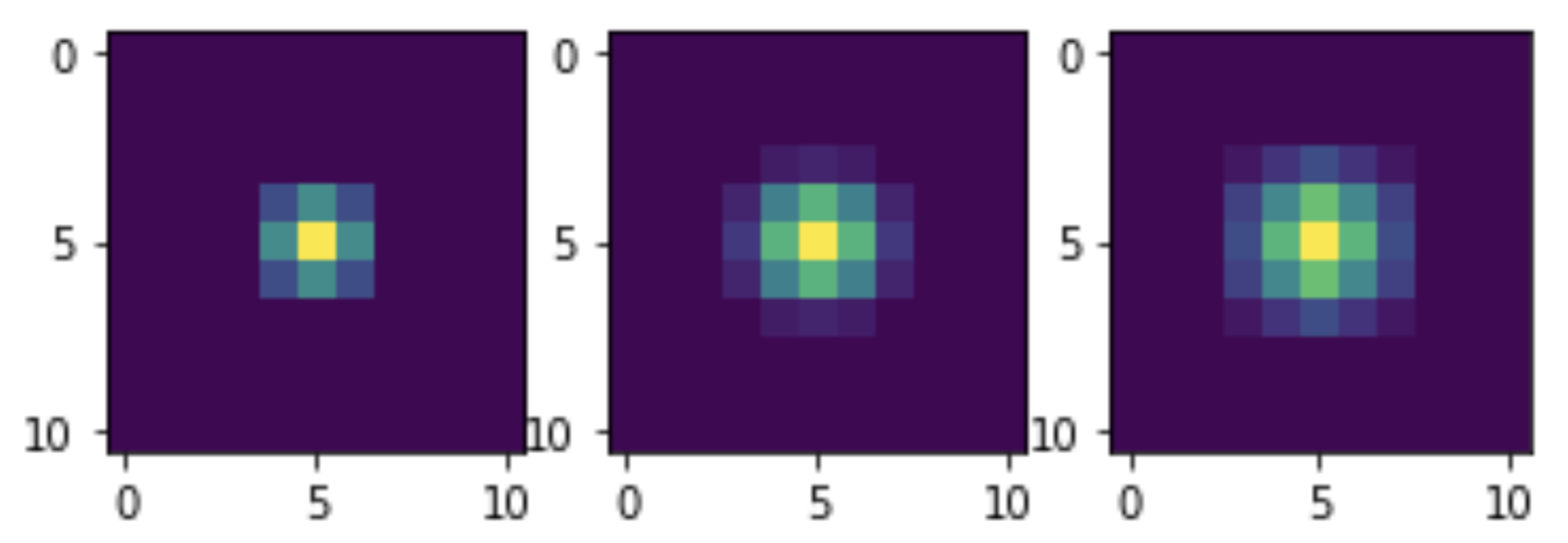
Now let's see the convolution with which kernels our filtering is equivalent. To do this, we will subject a single unit impulse to similar transformations and visualize. In fact, the impulse will not be single, but equal in amplitude to 255, since the mixing itself is optimized for integer data. But this does not interfere with evaluating the general appearance of the nuclei:
M = np.zeros((11, 11)) M[5, 5] = 255 M1 = smooth(M) M2 = smooth(M1) M3 = smooth(M2) plt.subplot(1, 3, 1) plt.imshow(M1) plt.subplot(1, 3, 2) plt.imshow(M2) plt.subplot(1, 3, 3) plt.imshow(M3) plt.show()
We considered a far from complete set of NumPy features, I hope this was enough to demonstrate the full power and beauty of this tool!
<up>
All Articles