Import OpenStreetMap. From the binary source to the table in the database in a few steps
Usually, when someone talks about OSM, one of the web services pops up in their head, or an application like Maps.me, based on OSM data . In fact, the OSM project is primarily data, everything else is essentially a special case of their use. Services usually provide only a portion of the information drawn according to their rules.
Initially, OSM is a collection of points, links between points, and tags for them. Community sources come in two formats. Initially, XML was used as a priority way of distributing data, but the Planet.osm file in uncompressed form has already exceeded terabytes, and I see no reason to use it for relatively voluminous information. PBF has a big advantage - it is binary and the entire earth file has a size of about 50GB (XML compressed about 80 GB).
It will be about importing OSM data from the “native” format using the Osmosis tool.
We also need PostgreSql with the Postgis extension, into which we will import OSM data.
As a result, it is possible to obtain information on objects with the tags listed here in their database .
First, create a database in Postgresql, the name does not really matter.
Next, add the extensions necessary for further work.
The Postgis extension "connects" to the database the actual module for working with geodata (I remind you that you must install Postgis itself). The hstore extension is designed to work with key / value sets, as a lot of information will be contained in OSM tags.
Download Osmosis . In short, it is software for a wide variety of operations with OSM data. There is some good documentation on working with the command line. Sources in Java. Below we will use the command line. I also used Osmosis as a Java library, the source code (available on GitHub) seemed clear enough to me, and the API was easy to use.
Now we are preparing the database for import. The necessary tables and functions can be created using scripts that are located in the osmosis / script folder. In addition to the main script, we will execute SQL code that will create a field for storing the geometry of the lines. This is due to the fact that OSM data is more likely represented as point connections than as a set of geometric shapes.
Well, now almost everything is ready. You can even run the import. It is necessary to decide what we will take as the source. Namely, you need to choose the format and source. Initially, the OSM community used (and uses) the XML format. But, the amount of data is growing and growing, so the text format is gradually being crowded out. Using PBF is somewhat more convenient. The central source planet.openstreetmap.org contains data for the entire globe. With one file you can download the entire knowledge base of the project, which has already exceeded 40 gigabytes in binary form. In those cases when I wanted to cut out a piece of data from there, I usually left the laptop working all night, providing it with more than 100GB of free space on the SSD for temporary files.
In our case, we can start by using uploads from community members. There are resources that make it possible to download data only for a specific region. For example, download.geofabrik.de . Take the Voronezh region. There it is included in a file containing data for the entire central federal district. You can download central-fed-district-latest.osm.pbf, and then cut the desired “piece” into a separate file or filter by coordinates when importing to the database. I would suggest the first option:
Everything is simple here. We read the PBF file, filter the reading results by the rectangle of coordinates, and write the results after filtering to the output file. You can filter by coordinates more accurately using not a rectangle, but a polygon whose coordinates are in a separate file.
The resulting file voronezh.osm.pbf is then imported into the database. To connect, create a properties file with database access parameters:
Well, the import itself:
Now you can already begin to study what we have in the database. The first thought is that there is a set of figures, but this is not entirely true. As I said, the main element is the point. Everything else is created by creating links (relationships) between points. We will not go deep yet, especially since the hands are already itching to create their own “flat” table with some data. Well, everything is ready for lines and points, you just need to create a table with the necessary fields, and insert the necessary entries there. And what fields do we have? Here to help the wiki. For example, take the key / value pair power = line . Choose a list of fields that we will use, for example: name, voltage, operator, cables. It turns out that we want to select the lines that necessarily have the power = line property, along with the fields name, voltage, operator, cables. Create a table:
And the request itself to fill out our new table:
Done, we have a table with power lines, where some lines even have some of the fields filled! Well, the table is certainly interesting, but visualizing the data to view the geometry would also be nice. The fastest way to do this is with QGIS, except that this powerful GIS must first be installed. There we already add a Postgis layer, use any map as a substrate (you can use the OpenLayers plugin). Configured, look:

Hurrah! Even very similar to the truth, I thought, looking out the window at the power lines.
And polygons?
The situation with dots is practically the same, except that you need to use the nodes table. KDPV just contains data on substations . And what about the polygons? Polygons also consist of lines (closed). It seems that you can just close the lines and enjoy the result, but it won’t work out that way. There are many pitfalls. Polygons can consist of several closed lines.
For example, an island may be on a lake. Therefore, we get a “hole” in the landfill. I also had to learn about the meaning of the word “exclave” (to my shame, I knew only about the “enclave”). Polygons are also grouped. For example, a forest may consist of several “pieces”. Which we should represent as one object. To top it all off, we must cut open polygons if some of the data is outside the map. I solved these, and some other other problems in the SQL script, which I safely put on the shelf after it worked. The osmosis-multypolygon project was found on GitHub. Reluctantly, I decided that using this solution is a better option than my set of scripts written on my knee in a couple of days. We do as it is said in README, namely, we execute a list of scripts, and we have a multipolygons table, which is filled with the instruction from assemble.sql. After we filled out the table with polygons, you can come up with what we want to get. Let's choose the territory of the parks ?
We look at the wiki and write a script:
Now we visualize:
Well, to be honest, here you can argue about the relevance of the data. But this is a topic for another discussion.
Initially, OSM is a collection of points, links between points, and tags for them. Community sources come in two formats. Initially, XML was used as a priority way of distributing data, but the Planet.osm file in uncompressed form has already exceeded terabytes, and I see no reason to use it for relatively voluminous information. PBF has a big advantage - it is binary and the entire earth file has a size of about 50GB (XML compressed about 80 GB).
It will be about importing OSM data from the “native” format using the Osmosis tool.
We also need PostgreSql with the Postgis extension, into which we will import OSM data.
As a result, it is possible to obtain information on objects with the tags listed here in their database .
DB preparation.
First, create a database in Postgresql, the name does not really matter.
psql -c "CREATE DATABASE map;"
Next, add the extensions necessary for further work.
psql -d map -c "CREATE EXTENSION postgis; CREATE EXTENSION hstore; "
The Postgis extension "connects" to the database the actual module for working with geodata (I remind you that you must install Postgis itself). The hstore extension is designed to work with key / value sets, as a lot of information will be contained in OSM tags.
Download Osmosis . In short, it is software for a wide variety of operations with OSM data. There is some good documentation on working with the command line. Sources in Java. Below we will use the command line. I also used Osmosis as a Java library, the source code (available on GitHub) seemed clear enough to me, and the API was easy to use.
Now we are preparing the database for import. The necessary tables and functions can be created using scripts that are located in the osmosis / script folder. In addition to the main script, we will execute SQL code that will create a field for storing the geometry of the lines. This is due to the fact that OSM data is more likely represented as point connections than as a set of geometric shapes.
psql -d map -fc:\osmosis\script\pgsnapshot_schema_0.6.sql psql -d map -fc:\osmosis\script\pgsnapshot_schema_0.6_linestring.sql
Import OSM data into a database
Well, now almost everything is ready. You can even run the import. It is necessary to decide what we will take as the source. Namely, you need to choose the format and source. Initially, the OSM community used (and uses) the XML format. But, the amount of data is growing and growing, so the text format is gradually being crowded out. Using PBF is somewhat more convenient. The central source planet.openstreetmap.org contains data for the entire globe. With one file you can download the entire knowledge base of the project, which has already exceeded 40 gigabytes in binary form. In those cases when I wanted to cut out a piece of data from there, I usually left the laptop working all night, providing it with more than 100GB of free space on the SSD for temporary files.
In our case, we can start by using uploads from community members. There are resources that make it possible to download data only for a specific region. For example, download.geofabrik.de . Take the Voronezh region. There it is included in a file containing data for the entire central federal district. You can download central-fed-district-latest.osm.pbf, and then cut the desired “piece” into a separate file or filter by coordinates when importing to the database. I would suggest the first option:
c:\osmosis\bin\osmosis.bat --read-pbf file="c:\downloads\central-fed-district-latest.osm.pbf" --bounding-box top=52.059564 left=37.92290 bottom=49.612297 right=43.225858 --write-pbf file="c:\map\voronezh.osm.pbf"
Everything is simple here. We read the PBF file, filter the reading results by the rectangle of coordinates, and write the results after filtering to the output file. You can filter by coordinates more accurately using not a rectangle, but a polygon whose coordinates are in a separate file.
The resulting file voronezh.osm.pbf is then imported into the database. To connect, create a properties file with database access parameters:
host=localhost database=map user=pguser password=pgpassword dbType=postgresql
Well, the import itself:
c:\osmosis\bin\osmosis.bat --read-pbf c:\map\voronezh.osm.pbf --write-pgsql authFile=c:\map\databaseinfo.properties
Imported Data
Now you can already begin to study what we have in the database. The first thought is that there is a set of figures, but this is not entirely true. As I said, the main element is the point. Everything else is created by creating links (relationships) between points. We will not go deep yet, especially since the hands are already itching to create their own “flat” table with some data. Well, everything is ready for lines and points, you just need to create a table with the necessary fields, and insert the necessary entries there. And what fields do we have? Here to help the wiki. For example, take the key / value pair power = line . Choose a list of fields that we will use, for example: name, voltage, operator, cables. It turns out that we want to select the lines that necessarily have the power = line property, along with the fields name, voltage, operator, cables. Create a table:
CREATE TABLE power_lines ( name varchar, voltage varchar, operator varchar, cables varchar, geom geometry )
And the request itself to fill out our new table:
INSERT INTO power_lines SELECT ways.tags -> 'name' as name, ways.tags -> 'voltage' as voltage, ways.tags -> 'operator' as operator, ways.tags -> 'cables' as cables, ways.linestring as geom FROM ways WHERE ways.tags -> 'power' IN ( 'line' )
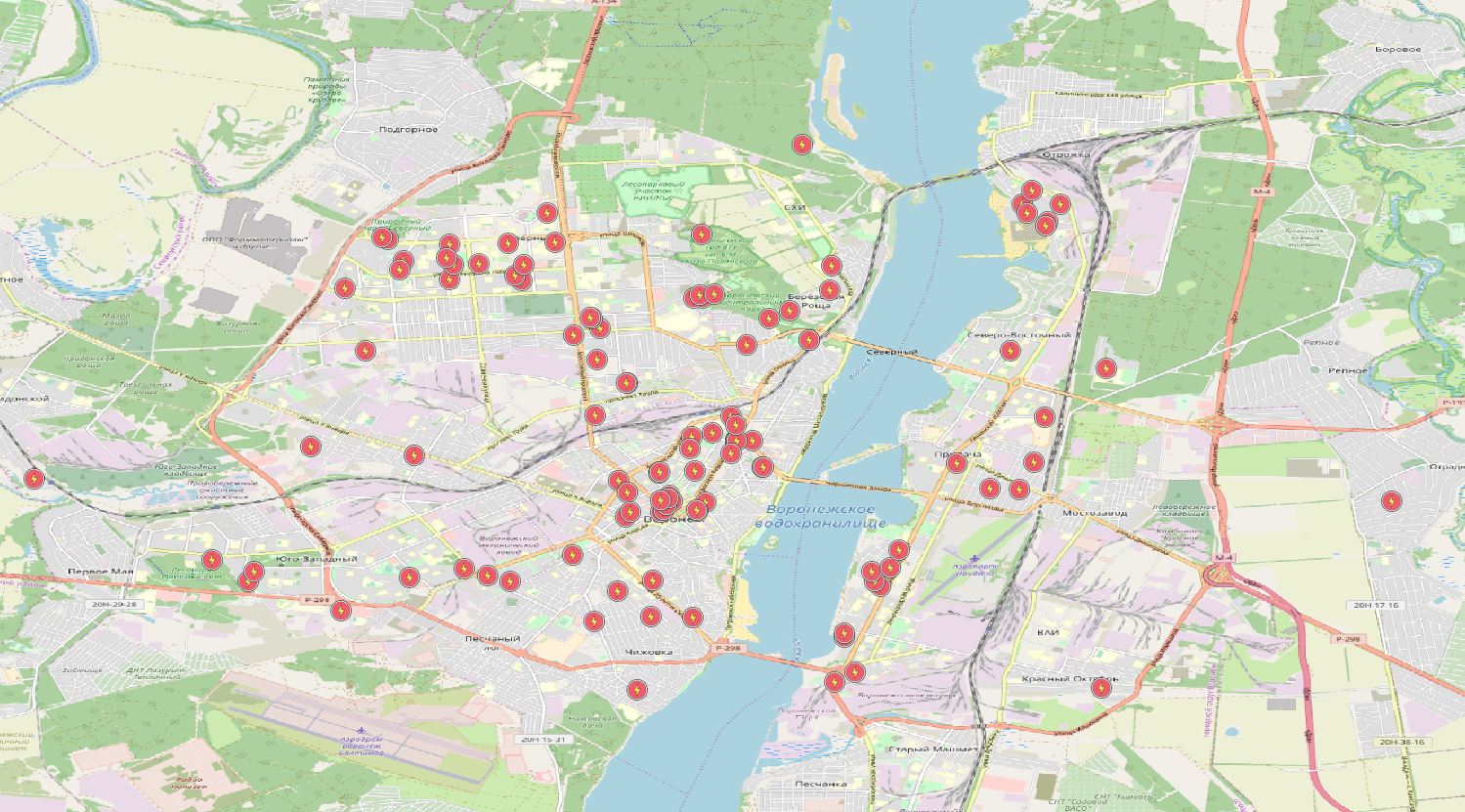
Done, we have a table with power lines, where some lines even have some of the fields filled! Well, the table is certainly interesting, but visualizing the data to view the geometry would also be nice. The fastest way to do this is with QGIS, except that this powerful GIS must first be installed. There we already add a Postgis layer, use any map as a substrate (you can use the OpenLayers plugin). Configured, look:
Hurrah! Even very similar to the truth, I thought, looking out the window at the power lines.
And polygons?
The situation with dots is practically the same, except that you need to use the nodes table. KDPV just contains data on substations . And what about the polygons? Polygons also consist of lines (closed). It seems that you can just close the lines and enjoy the result, but it won’t work out that way. There are many pitfalls. Polygons can consist of several closed lines.
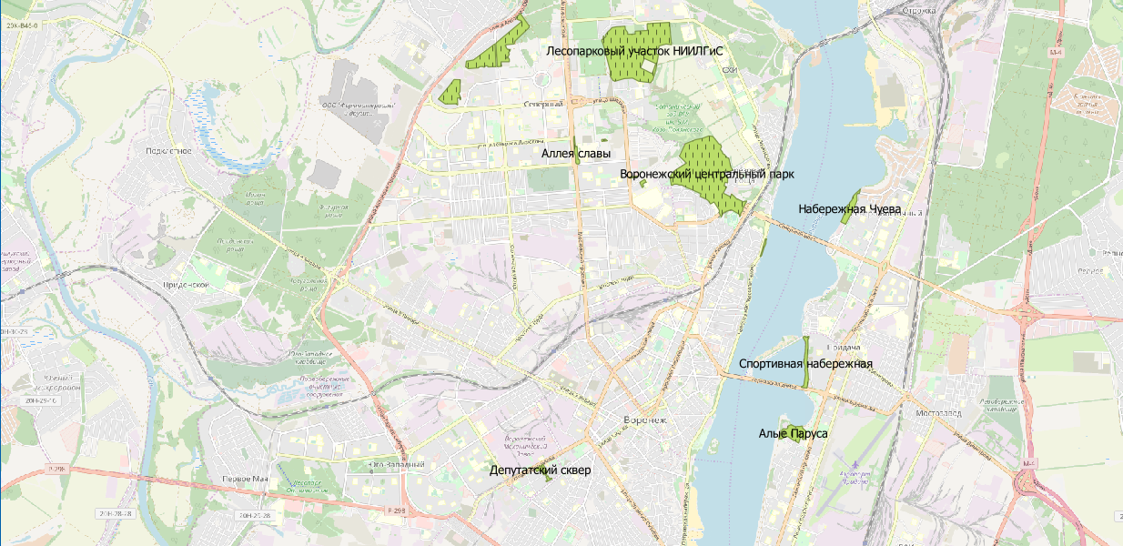
For example, an island may be on a lake. Therefore, we get a “hole” in the landfill. I also had to learn about the meaning of the word “exclave” (to my shame, I knew only about the “enclave”). Polygons are also grouped. For example, a forest may consist of several “pieces”. Which we should represent as one object. To top it all off, we must cut open polygons if some of the data is outside the map. I solved these, and some other other problems in the SQL script, which I safely put on the shelf after it worked. The osmosis-multypolygon project was found on GitHub. Reluctantly, I decided that using this solution is a better option than my set of scripts written on my knee in a couple of days. We do as it is said in README, namely, we execute a list of scripts, and we have a multipolygons table, which is filled with the instruction from assemble.sql. After we filled out the table with polygons, you can come up with what we want to get. Let's choose the territory of the parks ?
We look at the wiki and write a script:
CREATE TABLE parks ( name varchar, geom geometry ); INSERT INTO parks SELECT m.tags -> 'name' as name, m.geom FROM multipolygons m WHERE m.tags -> 'leisure' IN ( 'park' )
Now we visualize:
Well, to be honest, here you can argue about the relevance of the data. But this is a topic for another discussion.
All Articles