Neural networks and deep learning: an online tutorial, chapter 6, part 1: deep learning
Content
In the last chapter, we learned that deep neural networks (GNSs) are often harder to train than shallow ones. And this is bad, because we have every reason to believe that if we could train the STS, they would be much better at doing the tasks. But while the news from the previous chapter is disappointing, it won’t stop us. In this chapter, we will develop techniques that we can use to train deep networks and put them into practice. We will also look at the situation broader, briefly get acquainted with the recent progress in the use of GNS for image recognition, speech and for other applications. And also superficially consider what future the neural networks and AI can expect.
This will be a long chapter, so let's go over the table of contents a bit. Its sections are not strongly interconnected, therefore, if you have some basic concepts about neural networks, you can start with the section that interests you more.
The main part of the chapter is an introduction to one of the most popular types of deep networks: deep convolution networks (GSS). We will work with a detailed example of the use of a convolution network, with a code and other things, to solve the problem of classifying handwritten digits from the MNIST data set:
We begin our review of convolutional networks with shallow networks, which we used to solve this problem earlier in the book. In several stages we will create more and more powerful networks. Along the way, we will get to know many powerful technologies: convolutions, pooling, using GPUs to seriously increase the amount of training compared to what we did with shallow networks, algorithmic expansion of training data (to reduce overfitting), using dropout technology (also to reduce retraining), using ensembles of networks, and others. As a result, we will come to a system whose abilities are almost at the human level. Of the 10,000 MNIST verification images — which the system did not see during training — it will be able to correctly recognize 9967. And here are some of those images that were not recognized correctly. In the upper right corner are the correct options; what our program showed is indicated in the lower right corner.

Many of them are difficult to classify to humans. Take, for example, the third digit on the top line. It seems to me more like "9" than the official version of "8". Our network also decided that it was "9". At least, such errors can be fully understood, and perhaps even approved. We conclude our discussion of image recognition with an overview of the stunning progress that the neural networks (in particular, convolutional) have made recently.
The remainder of the chapter is devoted to a discussion of deep learning from a broader and less detailed point of view. We will briefly consider other NS models, in particular, recurrent NSs, and units of long-term short-term memory, and how these models can be used to solve problems in speech recognition, natural language processing, and others. We will discuss the future of NS and Civil Defense, from ideas such as intention-driven user interfaces to the role of deep learning in AI.
This chapter is based on material from previous chapters of the book, using and integrating ideas such as backpropagation, regularization, softmax, and so on. However, to read this chapter, it is not necessary to elaborate on the material of all previous chapters. However, it does not hurt to read Chapter 1 , and learn about the basics of the National Assembly. When I use the concepts from Chapters 2 through 5, I will give the necessary links to the material as necessary.
It is worth noting that this chapter does not. This is not training material on the latest and coolest libraries for working with NS. We are not going to train STS with dozens of layers to solve problems from the cutting edge of research. We will try to understand some of the basic principles that underlie GNS and apply them to the simple and easy-to-understand context of MNIST tasks. In other words, this chapter will not take you to the forefront of the region. The desire of this and the previous chapters is to concentrate on the basics, and prepare you to understand a wide range of contemporary works.
Introduction to convolutional neural networks
In the previous chapters, we taught our neural networks that it is pretty good to recognize images of handwritten numbers:
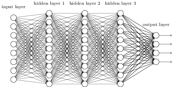
We did this using networks in which neighboring layers were completely connected to each other. That is, each neuron of the network was associated with each neuron of the neighboring layer:
In particular, we encoded the intensity of each pixel in the image as a value for the corresponding neuron of the input layer. For images 28x28 pixels in size, this means that the network will have 784 (= 28 × 28) incoming neurons. Then we trained the weights and offsets of the network so that at the output the network (there was such a hope) correctly identified the incoming image: '0', '1', '2', ..., '8', or '9'.
Our early networks work quite well: we achieved classification accuracy above 98% using training and verification data from the MNIST handwritten digits. But if you evaluate this situation now, it seems strange to use a network with fully connected layers to classify images. The fact is that such a network does not take into account the spatial structure of images. For example, it applies exactly the same to pixels located far from each other, as well as to neighboring pixels. It is assumed that conclusions about such spatial structure concepts should be made based on the study of training data. But what if, instead of starting the network structure from scratch, we will use an architecture trying to take advantage of the spatial structure? In this section I will describe convolutional neural networks (SNA). They use a special architecture, especially suitable for classifying images. Through the use of such an architecture, the SNA learns faster. And this helps us train deeper and layered networks that do a good job of classifying images. Today, deep SNA or a variant close to them is used in most cases of image recognition.
The origins of the SNA go back to the 1970s. But the starting work, which began their modern distribution, was the work of 1998, " Gradient Learning for Recognizing Documents ." Lekun made an interesting remark about the terminology used in the SNA: “The connection of models such as convolutional networks with neurobiology is very superficial. Therefore, I call them convolutional networks, not convolutional neural networks, and therefore we call their nodes elements, not neurons. " But, despite this, the SNA uses many ideas from the NS world that we have already studied: back propagation, gradient descent, regularization, nonlinear activation functions, etc. Therefore, we will follow the generally accepted agreement and consider them a kind of NA. I will call them both networks and neural networks, and their nodes - both neurons and elements.
SNA uses three basic ideas: local receptive fields, total weights, and pooling. Let's take a look at these ideas in turn.
Local receptive fields
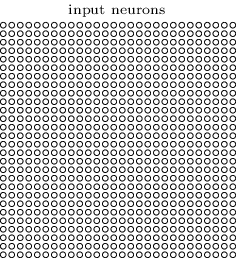
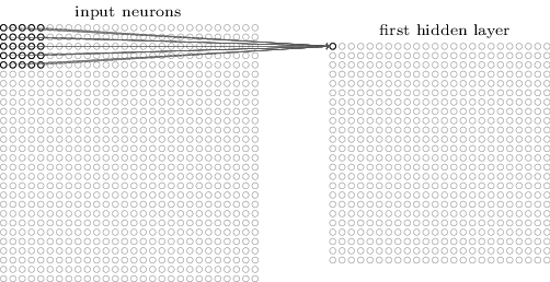
In fully connected network layers, input layers are indicated by vertical lines of neurons. In the SNA, it is more convenient to represent the input layer as a square of neurons with a dimension of 28x28, the values of which correspond to the pixel intensities of the image 28x28:
As usual, we associate incoming pixels with a layer of hidden neurons. However, we will not associate every pixel with every hidden neuron. We organize communications in small, localized areas of the incoming image.
More precisely, each neuron of the first hidden layer will be associated with a small portion of incoming neurons, for example, a 5x5 region corresponding to 25 incoming pixels. So, for some hidden neuron, the connection may look like this:
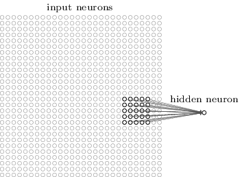
This portion of the incoming image is called the local receptive field for this hidden neuron. This is a small window looking at the incoming pixels. Each bond learns its own weight. Also, a hidden neuron studies general displacement. We can assume that this particular neuron is learning to analyze its specific local receptive field.
Then we move the local receptive field throughout the incoming image. Each local receptive field has its own hidden neuron in the first hidden layer. For a more specific illustration, start with the local receptive field in the upper left corner:
Move the local receptive field one pixel to the right (one neuron) to associate it with the second hidden neuron:
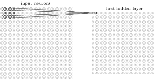
So we build the first hidden layer. Note that if our incoming image is 28x28 and the local receptive field is 5x5, then there will be 24x24 neurons in the hidden layer. This is because we can only move the local receptive field by 23 neurons to the right (or down), and then we will encounter the right (or bottom) side of the incoming image.
In this example, the local receptive fields move one pixel at a time. But sometimes a different step size is used. For example, we could shift the local receptive field 2 pixels to the side, and in this case we can talk about the size of step 2. In this chapter we will mainly use step 1, but you should know that sometimes experiments with steps of a different size are performed . You can experiment with the step size, as with other hyperparameters. You can also change the size of the local receptive field, but it usually turns out that a larger size of the local receptive field works better on images that are significantly larger than 28x28 pixels.
Total weights and offsets
I mentioned that each hidden neuron has an offset and 5x5 weights associated with its local receptive field. But I did not mention that we will use the same weights and displacements for all 24x24 hidden neurons. In other words, for a hidden neuron j, k, the output will be equal to:
Here σ is the activation function, possibly the sigmoid from the previous chapters. b is the total offset value. w l, m - array of total weights 5x5. And finally, a x, y denotes the input activation at position x, y.
This means that all neurons in the first hidden layer detect the same sign, just located in different parts of the image. A sign detected by a hidden neuron is a certain incoming sequence leading to the activation of a neuron: perhaps the edge of the image, or some form. To understand why this makes sense, suppose that our weights and displacements are such that a hidden neuron can recognize, say, a vertical face in a specific local receptive field. This ability is likely to be useful elsewhere in the image. Therefore, it is useful to use the same feature detector over the entire image area. More abstractly, the SNA is well adapted to the translational invariance of images: move the image, for example, of the cat, a little to the side, and it will still remain the image of the cat. True, the images from the MNIST digit classification problem are all centered and normalized in size. Therefore, MNIST has less translational invariance than random pictures. Still, features such as faces and angles are likely to be useful across the entire surface of the incoming image.
For this reason, sometimes we refer to the mapping of an incoming layer and a hidden layer as a feature map. Weights that define the characteristics map, we call total weights. And the bias defining the feature map is the general bias. It is often said that total weights and displacement determine the kernel or filter. But in literature people sometimes use these terms for a slightly different reason, and therefore I will not go deep into the terminology; better let's look at a few specific examples.
The network structure described by me is capable of recognizing only a localized attribute of one species. To recognize images, we need more feature maps. Therefore, the finished convolutional layer consists of several different feature maps:
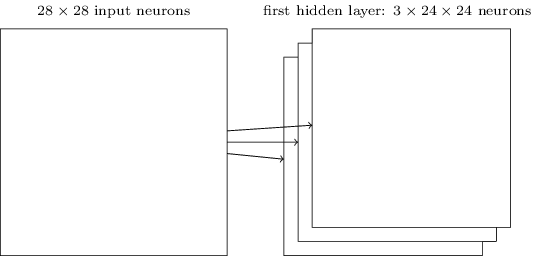
The example shows 3 feature maps. Each card is determined by a set of 5x5 total weights and one common offset. As a result, such a network can recognize three different types of signs, and each sign can be found in any part of the image.
I have drawn three feature cards for simplicity. In practice, the SNA can use more (possibly much more) feature maps. One of the early SNSs, LeNet-5, used 6 feature cards, each of which was associated with a 5x5 receptive field, to recognize MNIST digits. Therefore, the above example is very similar to LeNet-5. In the examples that we will independently develop further, we will use convolutional layers containing 20 and 40 feature cards. Let's take a quick look at the signs that we will examine:
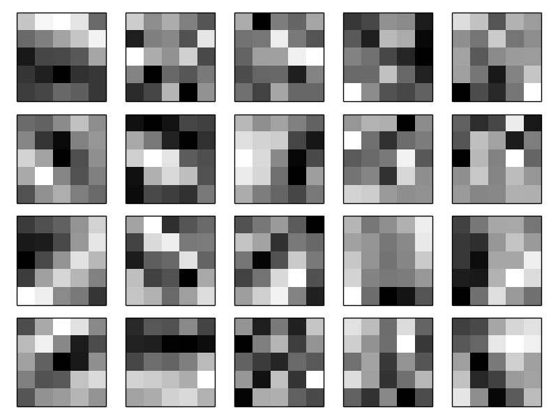
These 20 images correspond to 20 different attribute maps (filters, or kernels). Each card is represented by a 5x5 image corresponding to 5x5 weights of the local receptive field. White pixels mean low (usually more negative) weight, and the feature map reacts less to their corresponding pixels. Darker pixels mean more weight, and the feature map reacts more to their corresponding pixels. Roughly speaking, these images show those signs that the convolutional layer responds to.
What conclusions can be drawn from these attribute maps? Spatial structures here, obviously, did not appear in a random way - many signs show clear light and dark areas. This suggests that our network is really learning something related to spatial structures. However, besides this, it is rather difficult to understand what these signs are. We obviously do not study, say, Gabor filters , which were used in many traditional approaches to pattern recognition. In fact, a lot of work is being done now in order to better understand exactly which signs are studied by the SNA. If you are interested, I recommend starting with 2013 .
The big advantage of general weights and offsets is that this drastically reduces the number of parameters available to the SNA. For each feature map, we need 5 × 5 = 25 total weights and one common offset. Therefore, 26 parameters are required for each feature map. If we have 20 feature maps, then we will have 20 × 26 = 520 parameters that define the convolution layer. For comparison, suppose we have a fully connected first layer with 28 × 28 = 784 incoming neurons and relatively modest 30 hidden neurons - we used this scheme in many examples earlier. It turns out 784 × 30 weights, plus 30 offsets, a total of 23,550 parameters. In other words, a fully connected layer will have more than 40 times more parameters than a convolutional layer.
Of course, we cannot directly compare the number of parameters, since these two models differ radically. But intuitively it seems that using convolutional translational invariance reduces the number of parameters needed to achieve efficiency comparable to that of a fully connected model. And this, in turn, will accelerate the training of the convolutional model, and ultimately help us create deeper networks using convolutional layers.
By the way, the name “convolutional” comes from the operation in equation (125), which is sometimes called convolution . More precisely, sometimes people write this equation as a 1 = σ (b + w ∗ a 0 ), where a 1 denotes a set of output activations of one feature card, a 0 - a set of input activations, and * is called a convolution operation. We will not dig deep into the mathematics of convolutions, so you do not need to worry particularly about this connection. But it’s just worth knowing where the name came from.
Pooling layers
In addition to the convolutional layers described in the SNA, there are also pooling layers. They are usually used immediately after convolutional. They are committed to simplifying information from the output of the convolutional layer.
Here I use the phrase “feature map” not in the meaning of the function calculated by the convolutional layer, but to indicate the activation of the output of hidden layer neurons. Such free use of terms is often found in research literature.
The pooling layer accepts the output of each convolution layer feature map and prepares a compressed feature map. For example, each element of the pooling layer can summarize a section of, say, 2x2 neurons of the previous layer. Case study: One common pooling procedure is known as max pooling. In max-pooling, the pooling element simply gives the maximum activation from the 2x2 section, as shown in the diagram:
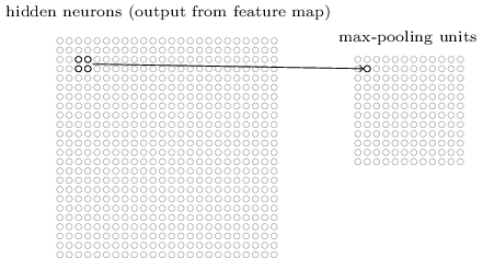
Since the output of convolutional layer neurons gives 24x24 values, after pulling we get 12x12 neurons.
As mentioned above, a convolutional layer usually implies something more than a single feature map. We apply max pooling to each feature map individually. So, if we have three feature cards, the combined convolution and max pooling layers will look like this:
Max-pulling can be imagined as a way of the network to ask if there is a given sign in any place of the image. And then she discards information about its exact location. It is intuitively clear that when a sign is found, its exact location is no longer as important as its approximate location relative to other signs. The advantage is that the number of features obtained by pooling is much smaller, and this helps to reduce the number of parameters required in the next layers.
Max pooling is not the only pooling technology. Another common approach is known as L2 pooling. In it, instead of taking the maximum activation of the 2x2 region of neurons, we take the square root of the sum of the squares of the activation of the 2x2 region. Details of the approaches differ, but intuitively it is similar to max-pooling: L2-pooling is a way to compress information from a convolutional layer. In practice, both technologies are often used. Sometimes people use other types of pooling. If you are struggling to optimize the quality of the network, you can use the supporting data to compare several different approaches to pulling, and choose the best one. But we will not worry about such a detailed optimization.
Summing up
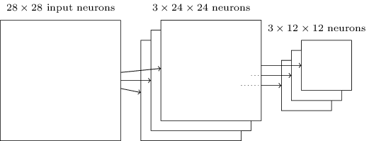
Now we can bring all the information together and get a complete SNA. It is similar to the architecture we recently reviewed, however, it has an additional layer of 10 output neurons corresponding to 10 possible values of the MNIST digits ('0', '1', '2', ..):
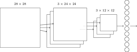
The network starts with 28x28 input neurons used to encode the pixel intensity of the MNIST image. After that comes a convolutional layer using local receptive fields 5x5 and 3 feature maps. The result is a layer of 3x24x24 hidden neurons of signs. The next step is a max pooling layer applied to 2x2 areas on each of the three feature maps. The result is a layer of 3x12x12 hidden traits neurons.
The last layer of connections in the network is fully connected. That is, it connects each neuron of the max pooling layer to each of the 10 output neurons. We used such a fully-connected architecture earlier. Note that in the diagram above, for simplicity, I used one arrow, not showing all the links. You can easily imagine them all.
This convolutional architecture is very different from what we used before. However, the overall picture is similar: a network consisting of many simple elements, whose behavior is determined by weights and offsets. The goal remains the same: use training data to train the network in weights and offsets so that the network classifies incoming numbers well.
In particular, as in the previous chapters, we will train our network using stochastic gradient descent and back propagation. The procedure goes almost the same as before. However, we need to make a few changes to the backpropagation procedure. The fact is that our derivatives for back propagation were intended for a network with fully connected layers. Fortunately, changing derivatives for convolutional and max-pooling layers is quite simple. If you want to understand the details, I invite you to try to solve the following problem. I’ll warn you that it will take a lot of time, unless you have thoroughly understood the early issues of differentiating backpropagation.
Task
- Reverse distribution in the convolution network. The main backpropagation equations in networks with fully connected layers are (BP1) - (BP4). Suppose our network contains a convolutional layer, a max-pooling layer and a fully connected output layer, as in the network described above. How do I change backpropagation equations?
Convolutional neural networks in practice
We discussed the ideas behind the SNA. Let's see how they work in practice by implementing some SNAs and applying them to the MNIST digit classification problem. We will use the network3.py program, an improved version of the network.py and network2.py programs created in previous chapters. The network3.py program uses ideas from Theano library documentation (in particular, LeNet-5 implementation ), from the implementation of an exception from Misha Denil and Chris Olah . The program code is available on GitHub.In the next section, we will study the code of the network3.py program, and in this section we will use it as a library for creating the SNA.
The network.py and network2.py programs were written in python using the Numpy matrix library. They worked on the basis of first principles, and reached the most detailed details of back propagation, stochastic gradient descent, etc. But now, when we understand these details, for network3.py we will use the Theano machine learning library (see the scientific work with its description). Theano is also the basis of the popular libraries for NS Pylearn2 and Keras , as well as Caffe and Torch .
Using Theano facilitates the implementation of backpropagation in the SNA, since it automatically counts all the cards. Theano is also noticeably faster than our previous code (which was written to facilitate understanding, and not for high-speed work), so it is reasonable to use it for training more complex networks. In particular, one of Theano's great features is to run code on both the CPU and GPU, if available. Running on a GPU provides a significant increase in speed, and helps train more complex networks.
To work in parallel with the book, you need to install Theano on your system. To do this, follow the instructions on the project home page. At the time of writing and launching the examples, Theano 0.7 was available. I ran some experiments on Mac OS X Yosemite without a GPU. Some on Ubuntu 14.04 with an NVIDIA GPU. And some are there, and there. To start network3.py, set the GPU flag in the code to True or False. In addition, the following instructions may help you to run Theano on your GPU . It’s also easy to find training materials online. If you don’t have your own GPU, you can look towards Amazon Web Services EC2 G2. But even with a GPU, our code will not work very quickly. Many experiments will go from a few minutes to several hours. The most complex of them on a single CPU will be executed for several days. As in the previous chapters, I recommend starting the experiment, and continue reading, periodically checking its operation. Without using a GPU, I recommend that you reduce the number of training eras for the most complex experiments.
To get basic results for comparison, let's start with a shallow architecture with one hidden layer containing 100 hidden neurons. We will study 60 eras, use the learning speed η = 0.1, the size of the mini-package 10, and we will study without regularization.
In this section, I set a specific number of training eras. I do this for clarity in the learning process. In practice, it is useful to use early stops, tracking the accuracy of the confirmation set, and stop training when we are convinced that the accuracy of confirmation is no longer improving:
>>> import network3 >>> from network3 import Network >>> from network3 import ConvPoolLayer, FullyConnectedLayer, SoftmaxLayer >>> training_data, validation_data, test_data = network3.load_data_shared() >>> mini_batch_size = 10 >>> net = Network([ FullyConnectedLayer(n_in=784, n_out=100), SoftmaxLayer(n_in=100, n_out=10)], mini_batch_size) >>> net.SGD(training_data, 60, mini_batch_size, 0.1, validation_data, test_data)
The best classification accuracy was 97.80%. This is the classification accuracy test_data, estimated from the training era, in which we got the best classification accuracy for data from validation_data. Using supporting evidence to make a decision about accuracy assessment helps to avoid retraining. Then we will do so. Your results may vary slightly, as network weights and offsets are randomly initialized.
The accuracy of 97.80% is pretty close to the accuracy of 98.04% obtained in Chapter 3, using similar network architecture and training hyperparameters. In particular, both examples use shallow networks with one hidden layer containing 100 hidden neurons. Both networks learn 60 eras with a mini-packet size of 10 and a learning rate of η = 0.1.
However, there were two differences in the earlier network. First, we performed regularization to help reduce the impact of retraining. Regularizing the current network improves accuracy, but not by much, so we won’t think about it for now. Secondly, although the last layer of the early network used sigmoid activations and the cross-entropy cost function, the current network uses the last layer with softmax, and the logarithmic likelihood function as a cost function. As described in chapter 3, this is not a major change. I did not switch from one to the other for some deep reason - mainly because softmax and the logarithmic likelihood function are more often used in modern networks to classify images.
Can we improve results using a deeper network architecture?
Let's start by inserting a convolutional layer, at the very beginning of the network. We will use the local receptive field 5x5, a step length of 1 and 20 feature cards. We will also insert a max pooling layer combining features using 2x2 pooling windows. So the overall network architecture will look similar to the one we discussed in the previous section, but with an additional fully connected layer:
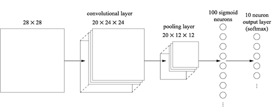
In this architecture, the convolution and pooling layers are trained in the local spatial structure contained in the incoming training picture, and the last, fully connected layer is trained at a more abstract level, integrating global information from the entire image. This is a commonly used scheme in the SNA.
Let's train such a network and see how it behaves.
>>> net = Network([ ConvPoolLayer(image_shape=(mini_batch_size, 1, 28, 28), filter_shape=(20, 1, 5, 5), poolsize=(2, 2)), FullyConnectedLayer(n_in=20*12*12, n_out=100), SoftmaxLayer(n_in=100, n_out=10)], mini_batch_size) >>> net.SGD(training_data, 60, mini_batch_size, 0.1, validation_data, test_data)
We get an accuracy of 98.78%, which is significantly higher than any of the previous results. We reduced the error by more than a third - an excellent result.
Describing the network structure, I considered convolutional and pooling layers as a single layer. To consider them as separate layers, or as a single layer - a matter of preference. network3.py considers them to be one layer, since the code is more compact. However, it is easy to modify network3.py so that the layers can be set individually.
Exercise
- What classification accuracy will we get if we lower the fully connected layer and use only the convolution / pool layer and the softmax layer? Does inclusion of a fully connected layer help?
Can we improve the result by 98.78%?
Let's try to insert the second convolution / pooling layer. We will insert it between the existing convolution / pooling and fully connected hidden layers. We again use the local 5x5 receptive field and the pool in 2x2 sections. Let's see what happens when we train a network with approximately the same hyperparameters as before:
>>> net = Network([ ConvPoolLayer(image_shape=(mini_batch_size, 1, 28, 28), filter_shape=(20, 1, 5, 5), poolsize=(2, 2)), ConvPoolLayer(image_shape=(mini_batch_size, 20, 12, 12), filter_shape=(40, 20, 5, 5), poolsize=(2, 2)), FullyConnectedLayer(n_in=40*4*4, n_out=100), SoftmaxLayer(n_in=100, n_out=10)], mini_batch_size) >>> net.SGD(training_data, 60, mini_batch_size, 0.1, validation_data, test_data)
And again, we have an improvement: now we get an accuracy of 99.06%!
At the moment, two natural questions arise. First: what does it mean to use the second convolution / pooling layer? You can assume that at the second convolution / pooling layer, “12x12” images come to the input, whose “pixels” represent the presence (or absence) of certain localized features in the original incoming picture. That is, we can assume that a certain version of the original incoming image comes to the input of this layer. This will be a more abstract and concise version, but it still has enough spatial structure, so it makes sense to use a second convolution / pulling layer to process it.
A pleasant point of view, but it raises a second question. At the output from the previous layer, 20 separate CPs are obtained, therefore 20x12x12 groups of input data come to the second convolution / pooling layer. It turns out that we have as if 20 separate images included in the convolution / pool layer, and not one image, as was the case with the first convolution / pool layer. How should neurons from the second convolution / pool layer respond to the multitude of these incoming images? In fact, we simply allow each neuron of this layer to be trained on the basis of all 20x5x5 neurons entering its local receptive field. In a less formal language, feature detectors in the second convolution / pool layer will have access to all features of the first layer, but only within their specific local receptive fields.
By the way, such a problem would have occurred in the first layer, if the images were color. In this case, we would have 3 input attributes per pixel, corresponding to the red, green and blue channels of the original image. And then we would also give sign detectors access to all color information, but only within the framework of their local receptive field.
Task
- Using the activation function in the form of hyperbolic tangent. Earlier in this book, I mentioned evidence several times that the tanh function, a hyperbolic tangent, might be better suited to be an activation function than a sigmoid. We did not do anything with this, since we had good progress with the sigmoid. But let's try some experiments with tanh as an activation function. Try to train a tang-activated network with convolutional and fully connected layers (you can pass activation_fn = tanh as a parameter to the ConvPoolLayer and FullyConnectedLayer classes). Start with the same hyperparameters that the sigmoid network had, but train the network of 20 eras, not 60. How does the network behave? What will happen if we continue until the 60th era? Try to build a graph of the accuracy of work confirmation by epoch for tangent and sigmoid, up to the 60th era. If your results are similar to mine, you will find that the tangent-based network learns a little faster, but the resulting accuracy of both networks is the same. Can you explain why this happens? Is it possible to achieve the same learning speed using a sigmoid - for example, by changing the learning speed or through scaling (remember that σ (z) = (1 + tanh (z / 2)) / 2)? Try five or six different hyperparameters or network architectures, look for where the tangent can be ahead of the sigmoid. I note that this task is open. Personally, I did not find any serious advantages in switching to the tangent, although I did not conduct comprehensive experiments, and perhaps you will find them. In any case, soon we will find an advantage in switching to a straightened linear activation function, so we will no longer delve into the issue of hyperbolic tangent.
Using straightened linear elements
The network that we have developed at the moment is one of the network options used in the fruitful work of 1998 , in which the task of MNIST, a network called LeNet-5, was first presented. This is a good basis for further experiments, to improve understanding of the issue and intuition. In particular, there are many ways in which we can change our network in search of ways to improve results.
First, let's change our neurons so that instead of using the sigmoid activation function, we can use straightened linear elements (ReLU). That is, we will use the activation function of the form f (z) ≡ max (0, z). We will train a network of 60 eras, with a speed of η = 0.03. I also found that it is a little more convenient to use the L2 regularization with the regularization parameter λ = 0.1:
>>> from network3 import ReLU >>> net = Network([ ConvPoolLayer(image_shape=(mini_batch_size, 1, 28, 28), filter_shape=(20, 1, 5, 5), poolsize=(2, 2), activation_fn=ReLU), ConvPoolLayer(image_shape=(mini_batch_size, 20, 12, 12), filter_shape=(40, 20, 5, 5), poolsize=(2, 2), activation_fn=ReLU), FullyConnectedLayer(n_in=40*4*4, n_out=100, activation_fn=ReLU), SoftmaxLayer(n_in=100, n_out=10)], mini_batch_size) >>> net.SGD(training_data, 60, mini_batch_size, 0.03, validation_data, test_data, lmbda=0.1)
I got a classification accuracy of 99.23%. A modest improvement over sigmoid results (99.06%). However, in all my experiments, I found that networks based on ReLU were ahead of networks based on the sigmoid activation function with enviable constancy. Apparently, there are real advantages in switching to ReLU to solve this problem.
What makes the ReLU activation function better than the sigmoid or hyperbolic tangent? At the moment, we do not particularly understand this. It is usually said that the function max (0, z) does not saturate at large z, in contrast to sigmoid neurons, and this helps ReLU neurons to continue learning. I don’t argue, but this justification cannot be called comprehensive, it’s just some kind of observation (I remind you that we discussed saturation in Chapter 2 ).
ReLU began to be actively used in the last few years. They were adopted for empirical reasons: some people tried ReLU, often simply based on hunches or heuristic arguments. They got good results, and the practice spread. In an ideal world, we would have a theory telling us which applications which activation functions are best for which applications. But for now, we still have a long way to go to such a situation. I would not be surprised at all if further improvements to the networks can be obtained by choosing some even more suitable activation function. I also expect that a good theory of activation functions will be developed in the coming decades. But today we have to rely on poorly studied rules of thumb and experience.
Expansion of training data
Another way that may possibly help us improve our results is to algorithmically expand the training data. The easiest way to expand the training data is to shift each training picture by one pixel, up, down, right or left. This can be done by running the expand_mnist.py program.
$ python expand_mnist.py
The launch of the program turns 50,000 training images of MNIST into an expanded set of 250,000 training images. Then we can use these training images to train the network. We will use the same network as before with ReLU. In my first experiments, I reduced the number of training eras - it made sense, because we have 5 times more training data. However, expanding the data set significantly reduced the effect of retraining. Therefore, after conducting several experiments, I returned to the number of eras 60. In any case, let's train:
>>> expanded_training_data, _, _ = network3.load_data_shared( "../data/mnist_expanded.pkl.gz") >>> net = Network([ ConvPoolLayer(image_shape=(mini_batch_size, 1, 28, 28), filter_shape=(20, 1, 5, 5), poolsize=(2, 2), activation_fn=ReLU), ConvPoolLayer(image_shape=(mini_batch_size, 20, 12, 12), filter_shape=(40, 20, 5, 5), poolsize=(2, 2), activation_fn=ReLU), FullyConnectedLayer(n_in=40*4*4, n_out=100, activation_fn=ReLU), SoftmaxLayer(n_in=100, n_out=10)], mini_batch_size) >>> net.SGD(expanded_training_data, 60, mini_batch_size, 0.03, validation_data, test_data, lmbda=0.1)
Using advanced training data, I got an accuracy of 99.37%. Such an almost trivial change provides a significant improvement in classification accuracy. And, as we discussed earlier, algorithmic data extension can be further developed. Just to remind you: in 2003, Simard, Steinkraus and Platt improved the accuracy of their network to 99.6%. Their network was similar to ours, they used two convolution / pool layers, followed by a fully connected layer with 100 neurons. The details of their architecture varied - they did not have the opportunity to take advantage of ReLU, for example - however, the key to improving the quality of work was the expansion of training data. They accomplished this by turning, transferring, and distorting MNIST training images. They also developed the “elastic distortion” process, emulating the random vibrations of the arm muscles while writing. By combining all these processes, they significantly increased the effective volume of their training data base, and due to this, achieved an accuracy of 99.6%.
Task
- The idea of convolutional layers is to work regardless of the location in the image. But then it may seem strange that our network is better trained when we simply shift the input images. Can you explain why this is actually quite reasonable?
Adding an Additional Fully Connected Layer
Is it possible to improve the situation? One of the possibilities is to use exactly the same procedure, but at the same time increase the size of the fully connected layer. I started the program with 300 and with 1000 neurons, and got results in 99.46% and 99.43%, respectively. This is interesting, but not particularly convincing than the previous result (99.37%).
What about adding an extra fully connected layer? Let's try adding an additional fully connected layer so that we have two hidden fully connected layers of 100 neurons:
>>> net = Network([ ConvPoolLayer(image_shape=(mini_batch_size, 1, 28, 28), filter_shape=(20, 1, 5, 5), poolsize=(2, 2), activation_fn=ReLU), ConvPoolLayer(image_shape=(mini_batch_size, 20, 12, 12), filter_shape=(40, 20, 5, 5), poolsize=(2, 2), activation_fn=ReLU), FullyConnectedLayer(n_in=40*4*4, n_out=100, activation_fn=ReLU), FullyConnectedLayer(n_in=100, n_out=100, activation_fn=ReLU), SoftmaxLayer(n_in=100, n_out=10)], mini_batch_size) >>> net.SGD(expanded_training_data, 60, mini_batch_size, 0.03, validation_data, test_data, lmbda=0.1)
Thus, I achieved verification accuracy of 99.43%. The expanded network again did not greatly improve performance. After conducting similar experiments with fully connected layers of 300 and 100 neurons, I got an accuracy of 99.48% and 99.47%. Inspirational, but not like a real win.
What's happening? Is it possible that extended or additional fully connected layers do not help in solving the MNIST problem? Or can our network achieve better, but we are developing it in the wrong direction? Maybe we could, for example, use tighter regularization to reduce retraining. One of the possibilities is the dropout technique mentioned in chapter 3. Recall that the basic idea of an exception is to randomly remove individual activations when training the network. As a result, the model becomes more resistant to the loss of individual evidence, and therefore it is less likely that it will rely on some small non-standard features of the training data. Let's try to apply the exception to the last fully connected layer:
>>> net = Network([ ConvPoolLayer(image_shape=(mini_batch_size, 1, 28, 28), filter_shape=(20, 1, 5, 5), poolsize=(2, 2), activation_fn=ReLU), ConvPoolLayer(image_shape=(mini_batch_size, 20, 12, 12), filter_shape=(40, 20, 5, 5), poolsize=(2, 2), activation_fn=ReLU), FullyConnectedLayer( n_in=40*4*4, n_out=1000, activation_fn=ReLU, p_dropout=0.5), FullyConnectedLayer( n_in=1000, n_out=1000, activation_fn=ReLU, p_dropout=0.5), SoftmaxLayer(n_in=1000, n_out=10, p_dropout=0.5)], mini_batch_size) >>> net.SGD(expanded_training_data, 40, mini_batch_size, 0.03, validation_data, test_data)
Using this approach, we achieve an accuracy of 99.60%, which is much better than the previous ones, especially our basic assessment - a network with 100 hidden neurons, which gives an accuracy of 99.37%.
Two changes are worth noting here.
First, I reduced the number of training eras to 40: exception reduces retraining, and we learn faster.
Secondly, fully connected hidden layers contain 1000 neurons, and not 100, as before. Of course, the exception, in fact, eliminates many neurons during training, so we should expect some kind of expansion. In fact, I conducted experiments with 300 and 1000 neurons, and received a slightly better confirmation in the case of 1000 neurons.
Using Network Ensemble
An easy way to improve efficiency is to create several neural networks and then get them to vote for a better classification. Suppose, for example, that we trained 5 different NS using the above recipe, and each of them achieved an accuracy close to 99.6%. Although all networks will show similar accuracy, they may have different errors due to different random initialization. It is reasonable to assume that if 5 NA vote, their general classification will be better than that of any network separately.
It sounds too good to be true, but assembling such ensembles is a common trick for both the National Assembly and other MO techniques. And it actually gives an improvement in efficiency: we get an accuracy of 99.67%. In other words, our network ensemble correctly classifies all 10,000 verification images, with the exception of 33.
The remaining errors are shown below. The label in the upper right corner is the correct classification according to MNIST data, and in the lower right corner is the label received by the network ensemble:
It is worthwhile to dwell on the images. The first two digits, 6 and 5 are the real mistakes of our ensemble. However, they can be understood, such a mistake could be made by man. This 6 is really very similar to 0, and 5 is very similar to 3. The third picture, supposedly 8, really looks more like 9. I side with the ensemble of networks: I think that he did the job better than the person who wrote this figure. On the other hand, the fourth image, 6, is really incorrectly classified by networks.
And so on. In most cases, the network solution seems plausible, and in some cases they better classified the figure than the person wrote it. On the whole, our networks are extremely effective, especially if we recall that they correctly classified 9967 images, which we do not present here.In this context, several obvious errors can be understood. Even a cautious person is sometimes mistaken. Therefore, I can expect a better result only from an extremely accurate and methodical person. Our network is approaching human performance.
Why did we apply the exception only to fully connected layers
If you look closely at the code above, you will see that we applied the exception only to fully connected network layers, but not to convolutional ones. In principle, a similar procedure can be applied to convolutional layers. But there is no need for this: convolutional layers have significant built-in resistance to retraining. This is because the total weights make the convolutional filters learn across the entire picture at once. As a result, they are less likely to trip over some local distortions in the training data. Therefore, there is no particular need to apply other regularizers to them, such as exceptions.
Moving on
You can improve the efficiency of solving the MNIST problem even more. Rodrigo Benenson put together an informative tablet that shows progress over the years, and provides links to work. Many of the works use GSS in the same way as we used them. If you rummage in your work, you will find many interesting techniques, and you may like to implement some of them. In this case, it would be wise to start their implementation with a simple network that can be quickly trained, and this will help you quickly begin to understand what is happening.
For the most part, I will not try to review recent work. But I can not resist one exception. It's about one work in 2010. I like her simplicity in her. The network is multilayer, and uses only fully connected layers (without convolutions). In their most successful network, there are hidden layers containing 2500, 2000, 1500, 1000 and 500 neurons, respectively. They used similar ideas to expand training data. But besides this, they applied several more tricks, including the lack of convolutional layers: it was the simplest, vanilla network, which, with proper patience and the availability of suitable computer capabilities, could have been taught back in the 1980s (if the MNIST set existed then). They achieved a classification accuracy of 99.65%, which roughly coincides with ours. The main thing in their work is the use of a very large and deep network, and the use of GPUs to accelerate learning. This allowed them to learn many eras. They also took advantage of the long length of training intervals,and gradually reduced the learning speed from 10-3 to 10 -6 . Trying to achieve similar results with an architecture like theirs is an interesting exercise.
Why do we get to learn?
In the previous chapter, we saw fundamental obstacles to learning deep multilayer NS. In particular, we saw that the gradient becomes very unstable: when moving from the output layer to the previous ones, the gradient tends to disappear (the problem of the disappearing gradient) or to explosive growth (the problem of explosive gradient growth). Since the gradient is the signal we use for training, this causes problems.
How did we manage to avoid them?
The answer, naturally, is this: we were not able to avoid them. Instead, we did a few things that allowed us to continue working, despite this. In particular: (1) the use of convolutional layers greatly reduces the number of parameters contained in them, greatly facilitating the learning problem; (2) the use of more efficient regularization techniques (exclusion and convolutional layers); (3) the use of ReLU instead of sigmoid neurons to accelerate learning - empirically up to 3-5 times; (4) the use of the GPU and the ability to learn over time. In particular, in recent experiments, we studied 40 eras using a data set 5 times larger than standard MNIST training data. Earlier in the book, we mainly studied 30 eras using standard training data. The combination of factors (3) and (4) gives such an effect,as if we studied 30 times longer than before.
You probably say, “Is that all?” Is that all it takes to train deep neural networks? And why then fuss fired up? ”
We, of course, used other ideas: big enough data sets (to help avoid retraining); correct cost function (to avoid learning slowdowns); good initialization of weights (also to avoid slowing down learning due to saturation of neurons); algorithmic extension of the training data set. We discussed these and other ideas in previous chapters, and usually we had the opportunity to reuse them with small notes in this chapter.
From all indications, this is a fairly simple set of ideas. Simple, however, capable of much when used in a complex. It turned out that getting started with deep learning was pretty easy!
?
If we consider convolution / pooling layers as one, then in our final architecture there are 4 hidden layers. Does such a network deserve a deep title? Naturally, 4 hidden layers are much more than in shallow networks that we studied earlier. Most networks had one hidden layer, sometimes 2. On the other hand, modern advanced networks sometimes have dozens of hidden layers. Sometimes I met people who thought that the deeper the network, the better, and that if you do not use a sufficiently large number of hidden layers, it means that you are not really doing deep learning. I don’t think so, in particular because such an approach turns the definition of deep learning into a procedure that depends on momentary results. A real breakthrough in this area was the idea of the practicality of going beyond networks with one or two hidden layers,prevailing in the mid 2000s. This was a real breakthrough, opening up a field of research with more expressive models. Well, a specific number of layers is not of fundamental interest. The use of deep networks is a tool to achieve other goals, such as improving classification accuracy.
Procedural issue
In this section, we smoothly switched from shallow networks with one hidden layer to multi-layer convolution networks. Everything seemed so easy! We made a change and got an improvement. If you start experimenting, I guarantee that usually everything will not go so smoothly. I presented you a combed story, omitting many experiments, including unsuccessful ones. I hope that this combed story will help you better understand the basic ideas. But he risks conveying an incomplete impression. Getting a good, working network requires a lot of trial and error, interspersed with frustration. In practice, you can expect a huge number of experiments. To speed up the process, the information in Chapter 3 regarding the selection of network hyperparameters, as well as the additional literature mentioned there, can help you.
Code for our convolution networks
Alright, let's now look at the code for our network3.py program. Structurally, it is similar to network2.py, which we developed in chapter 3, but the details are different due to the use of Theano library. Let's start with the FullyConnectedLayer class, similar to the layers we studied earlier.
class FullyConnectedLayer(object): def __init__(self, n_in, n_out, activation_fn=sigmoid, p_dropout=0.0): self.n_in = n_in self.n_out = n_out self.activation_fn = activation_fn self.p_dropout = p_dropout # Initialize weights and biases self.w = theano.shared( np.asarray( np.random.normal( loc=0.0, scale=np.sqrt(1.0/n_out), size=(n_in, n_out)), dtype=theano.config.floatX), name='w', borrow=True) self.b = theano.shared( np.asarray(np.random.normal(loc=0.0, scale=1.0, size=(n_out,)), dtype=theano.config.floatX), name='b', borrow=True) self.params = [self.w, self.b] def set_inpt(self, inpt, inpt_dropout, mini_batch_size): self.inpt = inpt.reshape((mini_batch_size, self.n_in)) self.output = self.activation_fn( (1-self.p_dropout)*T.dot(self.inpt, self.w) + self.b) self.y_out = T.argmax(self.output, axis=1) self.inpt_dropout = dropout_layer( inpt_dropout.reshape((mini_batch_size, self.n_in)), self.p_dropout) self.output_dropout = self.activation_fn( T.dot(self.inpt_dropout, self.w) + self.b) def accuracy(self, y): "Return the accuracy for the mini-batch." return T.mean(T.eq(y, self.y_out))
Most of the __init__ method speaks for itself, but a few notes can help clarify the code. As usual, we randomly initialize weights and offsets using normal random values with suitable standard deviations. These lines look a little incomprehensible. However, most of the weird code is loading weights and offsets into what the Theano library calls shared variables. This ensures that variables can be processed on the GPU, if available. We will not delve into this question - if interested, read the documentation for Theano. Also note that this initialization of weights and offsets is for the sigmoid activation function. Ideally, for functions like hyperbolic tangent and ReLU, we would initialize weights and offsets differently. This issue is discussed in future tasks.The __init__ method ends with the statement self.params = [self.w, self.b]. This is a convenient way to bring together all the learning parameters associated with a layer. Network.SGD later uses the params attributes to find out which variables in the Network class instance can be trained.
The set_inpt method is used to transfer input data to a layer and calculate the corresponding output. I write inpt instead of input because input is a built-in python function, and if you play with them, this can lead to unpredictable program behavior and difficult to diagnose errors. In fact, we pass input in two ways: through self.inpt and self.inpt_dropout. This is done as we may want to use exception during training. And then we will need to remove part of the self.p_dropout neurons. This is what the dropout_layer function in the penultimate line of the set_inpt method does. So, self.inpt_dropout and self.output_dropout are used during training, and self.inpt and self.output are used for all other purposes, for example, evaluating accuracy on validate and test data.
The class definitions for ConvPoolLayer and SoftmaxLayer are similar to FullyConnectedLayer. So similar that I won’t even quote the code. If you are interested, the full code of the program can be studied later in this chapter.
It is worth mentioning a couple of different details. Obviously, in ConvPoolLayer and SoftmaxLayer, we calculate the output activations in a way that suits the type of layer. Fortunately, Theano is easy to do, it has built-in operations for calculating convolution, max-pooling and the softmax function.
It’s less obvious how to initialize weights and offsets in the softmax layer - we did not discuss this. We mentioned that for sigmoidal weight layers, it is necessary to initialize appropriately parameterized normal random distributions. But this heuristic argument applied to sigmoid neurons (and, with minor corrections, to tang neurons). However, there is no particular reason for this argument to apply to softmax layers. Therefore, there is no reason to a priori apply this initialization again. Instead, I initialize all weights and offsets to 0. The option is spontaneous, but works pretty well in practice.
So, we have studied all the classes of layers. What about the Network class? Let's start by exploring the __init__ method:
class Network(object): def __init__(self, layers, mini_batch_size): """ layers, , mini_batch_size """ self.layers = layers self.mini_batch_size = mini_batch_size self.params = [param for layer in self.layers for param in layer.params] self.x = T.matrix("x") self.y = T.ivector("y") init_layer = self.layers[0] init_layer.set_inpt(self.x, self.x, self.mini_batch_size) for j in xrange(1, len(self.layers)): prev_layer, layer = self.layers[j-1], self.layers[j] layer.set_inpt( prev_layer.output, prev_layer.output_dropout, self.mini_batch_size) self.output = self.layers[-1].output self.output_dropout = self.layers[-1].output_dropout
Most of the code speaks for itself. The line self.params = [param for layer in ...] collects all the parameters for each layer into a single list. As previously suggested, the Network.SGD method uses self.params to figure out which parameters the Network can learn from. The lines self.x = T.matrix ("x") and self.y = T.ivector ("y") define the Theano x and y symbolic variables. They will represent the input and the desired output of the network.
This is not tutorial on using Theano, so I won’t go into what symbolic variables mean (see the documentation , and also one of the tutorials) Roughly speaking, they represent mathematical variables, not specific ones. With them, you can carry out many ordinary operations: add, subtract, multiply, apply functions, and so on. Theano provides many possibilities for manipulating such symbolic variables, convolving, max pulling, and so on. However, the main thing is the possibility of rapid symbolic differentiation using a very general form of the backpropagation algorithm. This is extremely useful for applying stochastic gradient descent to a wide range of network architectures. In particular, the following lines of code define the symbolic output of the network. We start by assigning the input to the first layer:
init_layer.set_inpt(self.x, self.x, self.mini_batch_size)
Input data is transmitted one mini-packet at a time, so its size is indicated there. We pass the self.x input two times: the fact is that we can use the network in two different ways (with or without exception). The for loop propagates the symbolic variable self.x through the Network layers. This allows us to define the final attributes output and output_dropout, which symbolically represent the output of the Network.
Having dealt with the initialization of Network, let's look at its training through the SGD method. The code looks long, but its structure is pretty simple. Explanations follow the code:
def SGD(self, training_data, epochs, mini_batch_size, eta, validation_data, test_data, lmbda=0.0): """ - .""" training_x, training_y = training_data validation_x, validation_y = validation_data test_x, test_y = test_data # - , num_training_batches = size(training_data)/mini_batch_size num_validation_batches = size(validation_data)/mini_batch_size num_test_batches = size(test_data)/mini_batch_size # , l2_norm_squared = sum([(layer.w**2).sum() for layer in self.layers]) cost = self.layers[-1].cost(self)+\ 0.5*lmbda*l2_norm_squared/num_training_batches grads = T.grad(cost, self.params) updates = [(param, param-eta*grad) for param, grad in zip(self.params, grads)] # - # -. i = T.lscalar() # mini-batch index train_mb = theano.function( [i], cost, updates=updates, givens={ self.x: training_x[i*self.mini_batch_size: (i+1)*self.mini_batch_size], self.y: training_y[i*self.mini_batch_size: (i+1)*self.mini_batch_size] }) validate_mb_accuracy = theano.function( [i], self.layers[-1].accuracy(self.y), givens={ self.x: validation_x[i*self.mini_batch_size: (i+1)*self.mini_batch_size], self.y: validation_y[i*self.mini_batch_size: (i+1)*self.mini_batch_size] }) test_mb_accuracy = theano.function( [i], self.layers[-1].accuracy(self.y), givens={ self.x: test_x[i*self.mini_batch_size: (i+1)*self.mini_batch_size], self.y: test_y[i*self.mini_batch_size: (i+1)*self.mini_batch_size] }) self.test_mb_predictions = theano.function( [i], self.layers[-1].y_out, givens={ self.x: test_x[i*self.mini_batch_size: (i+1)*self.mini_batch_size] }) # best_validation_accuracy = 0.0 for epoch in xrange(epochs): for minibatch_index in xrange(num_training_batches): iteration = num_training_batches*epoch+minibatch_index if iteration print("Training mini-batch number {0}".format(iteration)) cost_ij = train_mb(minibatch_index) if (iteration+1) validation_accuracy = np.mean( [validate_mb_accuracy(j) for j in xrange(num_validation_batches)]) print("Epoch {0}: validation accuracy {1:.2 epoch, validation_accuracy)) if validation_accuracy >= best_validation_accuracy: print("This is the best validation accuracy to date.") best_validation_accuracy = validation_accuracy best_iteration = iteration if test_data: test_accuracy = np.mean( [test_mb_accuracy(j) for j in xrange(num_test_batches)]) print('The corresponding test accuracy is {0:.2 test_accuracy)) print("Finished training network.") print("Best validation accuracy of {0:.2 best_validation_accuracy, best_iteration)) print("Corresponding test accuracy of {0:.2
The first lines are clear, they divide the data sets into components x and y, and calculate the number of mini-packets used in each data set. The following lines are more interesting, and they demonstrate why it is so interesting to work with Theano library. I will quote them here:
# , l2_norm_squared = sum([(layer.w**2).sum() for layer in self.layers]) cost = self.layers[-1].cost(self)+\ 0.5*lmbda*l2_norm_squared/num_training_batches grads = T.grad(cost, self.params) updates = [(param, param-eta*grad) for param, grad in zip(self.params, grads)]
In these lines, we symbolically define a regularized cost function based on the logarithmic likelihood function, calculate the corresponding derivatives in the gradient function, as well as the corresponding parameter updates. Theano allows us to do all this in just a few lines. The only thing hidden is that the calculation of the cost involves invoking the cost method for the output layer; this code is located elsewhere in network3.py. But it is short and simple. With the definition of all this, everything is ready to define the train_mb function, the Theano symbolic function that uses updates to update the Network parameters by the mini-packet index. Similarly, the validate_mb_accuracy and test_mb_accuracy functions calculate the Network accuracy on any given mini-packet of confirmation or verification data. Averaging over these functions,we can calculate accuracy on the entire validation and verification datasets.
The rest of the SGD method speaks for itself - we simply go through the epochs, training the network again and again on mini-packets of training data, and we calculate the accuracy of confirmation and verification.
Now we understand the most important parts of the year network3.py. Let's briefly go through the entire program. It is not necessary to study it all in detail, but you may like to go over the tops, and, perhaps, delve into some especially liked passages. But, of course, the best way to understand the program is to change it, add something new, refactor those parts that, in your opinion, can be improved. After the code, I present several tasks that contain a number of initial suggestions on what can be done here. Here is the code.
"""network3.py ~~~~~~~~~~~~~~ Theano . (, , -, softmax) (, , ReLU; ). CPU , network.py network2.py. , , GPU, . Theano, network.py network2.py. , . , API network2.py. , , . , , . Theano (http://deeplearning.net/tutorial/lenet.html ), (https://github.com/mdenil/dropout ) (http://colah.github.io ). Theano 0.6 0.7, . """ #### # import cPickle import gzip # import numpy as np import theano import theano.tensor as T from theano.tensor.nnet import conv from theano.tensor.nnet import softmax from theano.tensor import shared_randomstreams from theano.tensor.signal import downsample # def linear(z): return z def ReLU(z): return T.maximum(0.0, z) from theano.tensor.nnet import sigmoid from theano.tensor import tanh #### GPU = True if GPU: print "Trying to run under a GPU. If this is not desired, then modify "+\ "network3.py\nto set the GPU flag to False." try: theano.config.device = 'gpu' except: pass # it's already set theano.config.floatX = 'float32' else: print "Running with a CPU. If this is not desired, then the modify "+\ "network3.py to set\nthe GPU flag to True." #### MNIST def load_data_shared(filename="../data/mnist.pkl.gz"): f = gzip.open(filename, 'rb') training_data, validation_data, test_data = cPickle.load(f) f.close() def shared(data): """ . Theano GPU, . """ shared_x = theano.shared( np.asarray(data[0], dtype=theano.config.floatX), borrow=True) shared_y = theano.shared( np.asarray(data[1], dtype=theano.config.floatX), borrow=True) return shared_x, T.cast(shared_y, "int32") return [shared(training_data), shared(validation_data), shared(test_data)] #### class Network(object): def __init__(self, layers, mini_batch_size): """ layers, , mini_batch_size . """ self.layers = layers self.mini_batch_size = mini_batch_size self.params = [param for layer in self.layers for param in layer.params] self.x = T.matrix("x") self.y = T.ivector("y") init_layer = self.layers[0] init_layer.set_inpt(self.x, self.x, self.mini_batch_size) for j in xrange(1, len(self.layers)): prev_layer, layer = self.layers[j-1], self.layers[j] layer.set_inpt( prev_layer.output, prev_layer.output_dropout, self.mini_batch_size) self.output = self.layers[-1].output self.output_dropout = self.layers[-1].output_dropout def SGD(self, training_data, epochs, mini_batch_size, eta, validation_data, test_data, lmbda=0.0): """ - .""" training_x, training_y = training_data validation_x, validation_y = validation_data test_x, test_y = test_data # - , num_training_batches = size(training_data)/mini_batch_size num_validation_batches = size(validation_data)/mini_batch_size num_test_batches = size(test_data)/mini_batch_size # , l2_norm_squared = sum([(layer.w**2).sum() for layer in self.layers]) cost = self.layers[-1].cost(self)+\ 0.5*lmbda*l2_norm_squared/num_training_batches grads = T.grad(cost, self.params) updates = [(param, param-eta*grad) for param, grad in zip(self.params, grads)] # - # -. i = T.lscalar() # mini-batch index train_mb = theano.function( [i], cost, updates=updates, givens={ self.x: training_x[i*self.mini_batch_size: (i+1)*self.mini_batch_size], self.y: training_y[i*self.mini_batch_size: (i+1)*self.mini_batch_size] }) validate_mb_accuracy = theano.function( [i], self.layers[-1].accuracy(self.y), givens={ self.x: validation_x[i*self.mini_batch_size: (i+1)*self.mini_batch_size], self.y: validation_y[i*self.mini_batch_size: (i+1)*self.mini_batch_size] }) test_mb_accuracy = theano.function( [i], self.layers[-1].accuracy(self.y), givens={ self.x: test_x[i*self.mini_batch_size: (i+1)*self.mini_batch_size], self.y: test_y[i*self.mini_batch_size: (i+1)*self.mini_batch_size] }) self.test_mb_predictions = theano.function( [i], self.layers[-1].y_out, givens={ self.x: test_x[i*self.mini_batch_size: (i+1)*self.mini_batch_size] }) # best_validation_accuracy = 0.0 for epoch in xrange(epochs): for minibatch_index in xrange(num_training_batches): iteration = num_training_batches*epoch+minibatch_index if iteration % 1000 == 0: print("Training mini-batch number {0}".format(iteration)) cost_ij = train_mb(minibatch_index) if (iteration+1) % num_training_batches == 0: validation_accuracy = np.mean( [validate_mb_accuracy(j) for j in xrange(num_validation_batches)]) print("Epoch {0}: validation accuracy {1:.2%}".format( epoch, validation_accuracy)) if validation_accuracy >= best_validation_accuracy: print("This is the best validation accuracy to date.") best_validation_accuracy = validation_accuracy best_iteration = iteration if test_data: test_accuracy = np.mean( [test_mb_accuracy(j) for j in xrange(num_test_batches)]) print('The corresponding test accuracy is {0:.2%}'.format( test_accuracy)) print("Finished training network.") print("Best validation accuracy of {0:.2%} obtained at iteration {1}".format( best_validation_accuracy, best_iteration)) print("Corresponding test accuracy of {0:.2%}".format(test_accuracy)) #### class ConvPoolLayer(object): """ - . , , , . """ def __init__(self, filter_shape, image_shape, poolsize=(2, 2), activation_fn=sigmoid): """`filter_shape` - 4, , , . `image_shape` - 4, -, , . `poolsize` - 2, y x. """ self.filter_shape = filter_shape self.image_shape = image_shape self.poolsize = poolsize self.activation_fn=activation_fn # initialize weights and biases n_out = (filter_shape[0]*np.prod(filter_shape[2:])/np.prod(poolsize)) self.w = theano.shared( np.asarray( np.random.normal(loc=0, scale=np.sqrt(1.0/n_out), size=filter_shape), dtype=theano.config.floatX), borrow=True) self.b = theano.shared( np.asarray( np.random.normal(loc=0, scale=1.0, size=(filter_shape[0],)), dtype=theano.config.floatX), borrow=True) self.params = [self.w, self.b] def set_inpt(self, inpt, inpt_dropout, mini_batch_size): self.inpt = inpt.reshape(self.image_shape) conv_out = conv.conv2d( input=self.inpt, filters=self.w, filter_shape=self.filter_shape, image_shape=self.image_shape) pooled_out = downsample.max_pool_2d( input=conv_out, ds=self.poolsize, ignore_border=True) self.output = self.activation_fn( pooled_out + self.b.dimshuffle('x', 0, 'x', 'x')) self.output_dropout = self.output # no dropout in the convolutional layers class FullyConnectedLayer(object): def __init__(self, n_in, n_out, activation_fn=sigmoid, p_dropout=0.0): self.n_in = n_in self.n_out = n_out self.activation_fn = activation_fn self.p_dropout = p_dropout # Initialize weights and biases self.w = theano.shared( np.asarray( np.random.normal( loc=0.0, scale=np.sqrt(1.0/n_out), size=(n_in, n_out)), dtype=theano.config.floatX), name='w', borrow=True) self.b = theano.shared( np.asarray(np.random.normal(loc=0.0, scale=1.0, size=(n_out,)), dtype=theano.config.floatX), name='b', borrow=True) self.params = [self.w, self.b] def set_inpt(self, inpt, inpt_dropout, mini_batch_size): self.inpt = inpt.reshape((mini_batch_size, self.n_in)) self.output = self.activation_fn( (1-self.p_dropout)*T.dot(self.inpt, self.w) + self.b) self.y_out = T.argmax(self.output, axis=1) self.inpt_dropout = dropout_layer( inpt_dropout.reshape((mini_batch_size, self.n_in)), self.p_dropout) self.output_dropout = self.activation_fn( T.dot(self.inpt_dropout, self.w) + self.b) def accuracy(self, y): "Return the accuracy for the mini-batch." return T.mean(T.eq(y, self.y_out)) class SoftmaxLayer(object): def __init__(self, n_in, n_out, p_dropout=0.0): self.n_in = n_in self.n_out = n_out self.p_dropout = p_dropout # self.w = theano.shared( np.zeros((n_in, n_out), dtype=theano.config.floatX), name='w', borrow=True) self.b = theano.shared( np.zeros((n_out,), dtype=theano.config.floatX), name='b', borrow=True) self.params = [self.w, self.b] def set_inpt(self, inpt, inpt_dropout, mini_batch_size): self.inpt = inpt.reshape((mini_batch_size, self.n_in)) self.output = softmax((1-self.p_dropout)*T.dot(self.inpt, self.w) + self.b) self.y_out = T.argmax(self.output, axis=1) self.inpt_dropout = dropout_layer( inpt_dropout.reshape((mini_batch_size, self.n_in)), self.p_dropout) self.output_dropout = softmax(T.dot(self.inpt_dropout, self.w) + self.b) def cost(self, net): " ." return -T.mean(T.log(self.output_dropout)[T.arange(net.y.shape[0]), net.y]) def accuracy(self, y): " -." return T.mean(T.eq(y, self.y_out)) #### def size(data): " `data`." return data[0].get_value(borrow=True).shape[0] def dropout_layer(layer, p_dropout): srng = shared_randomstreams.RandomStreams( np.random.RandomState(0).randint(999999)) mask = srng.binomial(n=1, p=1-p_dropout, size=layer.shape) return layer*T.cast(mask, theano.config.floatX)
Tasks
All Articles