Differential geometry of curves. Part 1

Foreword

Hello to all readers. I just decided to write an article on differential geometry of curves. In my opinion, the topic of "continuous" mathematics will be useful to most Habr readers, at least for the next hour =), given that this is an IT resource, and IT is somewhere closer to discrete mathematics (again, in my imperfect view). But in some places, I know for sure there is not only a discrete one, for example, CAD design systems have engines built on differential geometry (well, of course, not just one, and computational geometry is there, and so on). Perhaps it’s used in games, I don’t know. After all, a game is usually a movement, and to describe a movement it would be nice to know the geometry.

Introduction

Differential geometry of curves (as the name implies) deals with the geometry of curves, but using methods of differential calculus, or matanalysis.



For those who set the curves only on the plane, in this form:

$$

$$y = ax + b$$

or the like:

$$

$$y = \ frac {1} {\ sigma \ sqrt {2 \ pi}} \ exp \ left (- \ frac {(x- \ mu) ^ 2} {2 \ sigma ^ 2} \ right)$$

even so (implicit task):

$$

$$y ^ {3} x = 7x ^ {2} + 4$$

I will say that this is not the best way, that is, it is not universal, but it may be inconvenient (for spaces of higher dimension). It is possible, of course, and so, it will be good for your tasks, but in general, the curves are set in parametric form. Because if you set this way already in 3D space, you get something like:

\ begin {equation *}

\ begin {cases}

z = 2x-y,

\\

z = x ^ {2} + y ^ {2}

\ end {cases}

\ end {equation *}

and even so:

\ begin {equation *}

\ begin {cases}

z = 2x-y,

\\

y = x ^ {2} + z ^ {2}

\ end {cases}

\ end {equation *}

What can be interpreted as the intersection of two arbitrary surfaces. It is the intersection that sets the spatial curve for us. And another circle example:

\ begin {equation *}

\ begin {cases}

x ^ {2} + y ^ {2} + z ^ {2} = 1,

\\

x + y + z = 1

\ end {cases}

\ end {equation *}



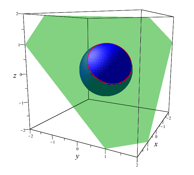
Picture for a better understanding of what happens when you cross



And you ask why these methods are similar. Well, look, in the plane we have in general the implicit specification of the curve $$$F (x, y) = 0.$ Then in 3D space, by analogy, I want to write down the equation by adding one coordinate $$$F (x, y, z) = 0.$ But all the same it turns out not a curve, but a surface. Then if you add another equation, you get a system, or two surfaces:

\ begin {equation}

\ begin {cases}

F (x, y, z) = 0,

\\

G (x, y, z) = 0.

\ end {cases}

\ end {equation}

which, generally speaking, may not intersect, because arbitrary $$$F$ and $$$G$ not always give a curve.



Therefore, let us rather move on to the parametric assignment of curves.

Curve Parametric

“Define a curve parametrically” means to specify the coordinate of each point on the curve. That is, each coordinate individually will be a function of the general parameter.

\ begin {equation *}

\ begin {cases}

x = x (t),

\\

y = y (t),

\\

z = z (t).

\ end {cases}

\ end {equation *}

This thing is usually called the radius vector. $$$\ vec {r} (t) = (x, y, z).$ Or, to be more precise, more correct as follows:

$$

$$\ vec {r} (t) = (x, y, z) ^ {T} = \ begin {bmatrix} x \\ y \\ z \ end {bmatrix}$$

A regular vector is a column vector, or a transposed row vector. If we go into the wilds of tensor analysis, then column vector = vector, and row vector = covector. But this does not matter to us, because anyway, in the orthogonal normalized basis, in which we work, the difference between them disappears. Next, I will write the vectors into a string, it does not affect anything, but compactly it turns out.



By the way, if you look at system 1, and for convenience, indicating, for example, $$$z = t$ :

\ begin {equation *}

\ begin {cases}

F (x, y, t) = 0,

\\

G (x, y, t) = 0.

\ end {cases}

\ end {equation *}

then formally solving this system of equations with respect to $$$x, y$ , we obtain a solution depending on the parameter $$$\ {x (t), y (t) \}$ . And now, if everything is combined into one vector:

\ begin {equation *}

\ begin {cases}

x = x (t),

\\

y = y (t),

\\

z = t

\ end {cases}

\ end {equation *}

we get some parameterization of the curve, until recently, given as the intersection of surfaces.



Well, for example, a helix:

\ begin {equation *}

\ begin {cases}

x = cos (t),

\\

y = sin (t),

\\

z = t

\ end {cases}

\ end {equation *}



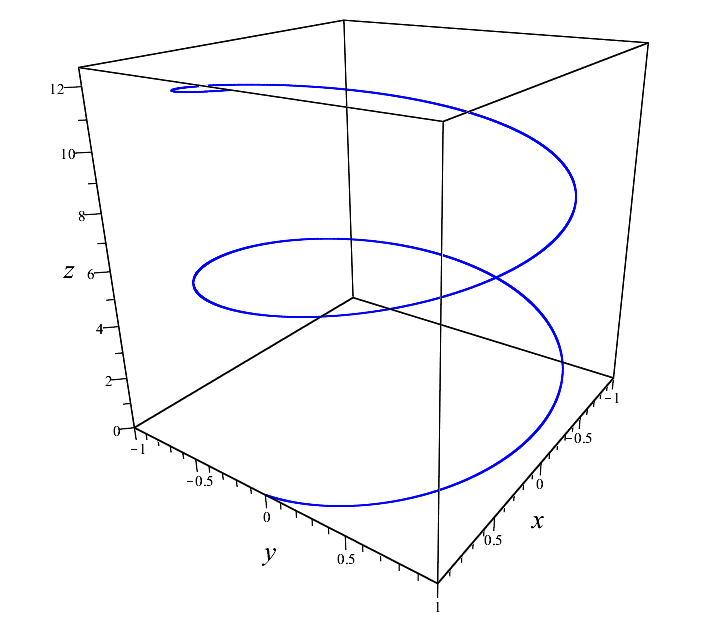
Helix



Here in the picture is the parameter $$$t$ runs over values ​​from $$$0$ before $$$4 \ pi$ . By the way, with the sentence earlier, I said “some parameterization”. And this is no accident. Because there can be infinitely many parametrizations of this particular helix.

For example, the same line:

\ begin {equation *}

\ begin {cases}

x = cos (t ^ {2}),

\\

y = sin (t ^ {2}),

\\

z = t ^ {2}

\ end {cases}

\ end {equation *}

this is the same helix, and the picture will be the same (I will not insert it again), however, $$$t$ runs over values ​​from $$$0$ before $$$2 \ sqrt {\ pi}$ .

Anyway, making a replacement $$$t = g (\ tilde {t})$ , it will be the same helix (provided that $$$g (\ tilde {t})$ - monotonous):

\ begin {equation *}

\ begin {cases}

x (\ tilde {t}) = cos (g (\ tilde {t})),

\\

y (\ tilde {t}) = sin (g (\ tilde {t})),

\\

z (\ tilde {t}) = g (\ tilde {t}).

\ end {cases}

\ end {equation *}

We will talk more about parameterization later, and about a special parameterization called “natural”, but already in the following articles (maybe).

Derivative and tangent vector

And now, it's time to start the differential analysis of the curves. Don’t worry, the definition of the derivative of the vector will slip quickly;) So, here we have a vector depending on the parameter $$$t$ : $$$\ vec {r} (t) = (x (t), y (t), z (t)).$

You can write it laid out on a basis: $$$\ vec {r} (t) = x (t) \ vec {i} + y (t) \ vec {j} + z (t) \ vec {k}$ .

And the derivative, as usual, is defined as the limit:

$$

$$\ dot {\ vec {r}} = \ frac {d \ vec {r}} {dt} = \ lim _ {\ Delta t \ to 0} \ frac {\ Delta \ vec {r}} {\ Delta t } = \ lim _ {\ Delta t \ to 0} \ frac {\ vec {r} (t + \ Delta t) - \ vec {r} (t)} {\ Delta t},$$

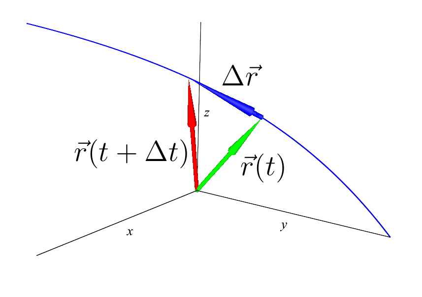
Derivative of a vector function (almost)



the limit of the vector function itself is the limits of each of the components:

\ begin {equation *}

\ dot {\ vec {r}} = \ lim _ {\ Delta t \ to 0} \ frac {[x (t + \ Delta t) \ vec {i} + y (t + \ Delta t) \ vec {j} + z (t + \ Delta t) \ vec {k}] - [x (t) \ vec {i} + y (t) \ vec {j} + z (t) \ vec {k}]} {\ Delta t } = \\

\ lim _ {\ Delta t \ to 0} \ frac {[x (t + \ Delta t) -x (t)] \ vec {i} + [y (t + \ Delta t) -y (t)] \ vec { j} + [z (t + \ Delta t) -z (t)] \ vec {k}]} {\ Delta t} = \\

\ lim _ {\ Delta t \ to 0} \ frac {x (t + \ Delta t) -x (t)} {\ Delta t} \ vec {i} + \ lim _ {\ Delta t \ to 0} ... = \ \ \ dot {x} \ vec {i} + \ dot {y} \ vec {j} + \ dot {z} \ vec {k} = (\ dot {x}, \ dot {y}, \ dot { z}).

\ end {equation *}

Well, even the figure shows where $$$\ Delta t$ not even rushed to zero that this vector $$$\ dot {\ vec {r}}$ is tangent to the curve. In the theory it is interpreted as speed and is designated as follows:

$$

$$\ dot {\ vec {r}} = \ vec {v},$$

and the curve itself, respectively, as the trajectory of the motion of the material point, but we will talk more about this later.

So, this vector $$$\ vec {v}$ is tangent to our curve everywhere except for singular points (in the sense that at singular points of the tangent vector it may not exist). But there are so few of them that let's not even talk about them yet. And it turns out that our vector $$$\ vec {v}$ there is a basis for our curve, it shows where the curve goes further. Therefore, it would be better to make it single as all other unit vectors. Just divide by its length and designate as usual:

$$

$$\ vec {\ tau} = \ frac {\ vec {v}} {v},$$

now then, it is always equal to one:

$$

$$\ langle \ vec {\ tau}, \ vec {\ tau} \ rangle = \ langle \ frac {\ vec {v}} {v}, \ frac {\ vec {v}} {v} \ rangle = \ frac {\ langle \ vec {v}, \ vec {v} \ rangle} {v ^ {2}} = \ frac {v ^ {2}} {v ^ {2}} = 1$$

Normal vector

And now, for the sake of fun, this equality can be differentiated, both the left and right sides (in general, in such matters, if you don’t meet anything, it’s better to differentiate just in case):

$$

$$\ frac {d \ langle \ vec {\ tau}, \ vec {\ tau} \ rangle} {dt} = \ frac {d (1)} {dt},$$

on the right, of course, zero. But on the left, we differentiate the scalar product of vectors. Given the rules of differentiation of scalar, vector products and other things (which are not at all difficult to prove, even having only what is written above in this article):

$$

$$\ frac {d \ langle \ vec {a}, \ vec {b} \ rangle} {dt} = \ langle \ dot {\ vec {a}}, \ vec {b} \ rangle + \ langle \ vec { a}, \ dot {\ vec {b}} \ rangle,$$

$$

$$\ frac {d [\ vec {a}, \ vec {b}]} {dt} = [\ dot {\ vec {a}}, \ vec {b}] + [\ vec {a}, \ dot {\ vec {b}}],$$

$$

$$\ frac {d (k \ vec {a})} {dt} = \ dot {k} \ vec {a} + k \ dot {\ vec {a}},$$

in the last expression $$$k = k (t)$ scalar function depending on the parameter.

Well now, let's finish the job without any problems:

$$

$$\ langle \ dot {\ vec {\ tau}}, \ vec {\ tau} \ rangle + \ langle \ vec {\ tau}, \ dot {\ vec {\ tau}} \ rangle = 0,$$

$$

$$2 \ langle \ vec {\ tau}, \ dot {\ vec {\ tau}} \ rangle = 0,$$

$$

$$\ langle \ vec {\ tau}, \ dot {\ vec {\ tau}} \ rangle = 0,$$

here we also took into account the symmetry property of the scalar product, and from there the two got out:

$$

$$\ langle \ vec {a}, \ vec {b} \ rangle = \ langle \ vec {b}, \ vec {a} \ rangle.$$

Well, now you can draw conclusions. The last scalar product is zero. And this happens only when either at least one of the vectors is zero, or they are perpendicular. Since our $$$\ vec {\ tau}$ completely arbitrary (why do we all do this? To calculate the tangent vector for absolutely any curve), we conclude that the derived vector from the unit tangent is always perpendicular to it, located at an angle $$$90 ^ {\ circ}$ :

$$

$$\ vec {\ tau} \ perp \ dot {\ vec {\ tau}}.$$

Fine. This derived vector can be called the normal vector to our curve. But we want him to be single too, and this is completely optional at the moment. Therefore, we simply divide by its length, then it certainly will not go anywhere:

$$

$$\ vec {n} = \ frac {\ dot {\ vec {\ tau}}} {| \ dot {\ vec {\ tau}} |}.$$

Remembering what is $$$\ vec {\ tau}$ , find its derivative:

$$

$$\ dot {\ vec {\ tau}} = \ frac {d \ vec {\ tau}} {dt} = \ frac {d} {dt} \ left (\ frac {\ vec {v}} {v} \ right),$$

here the differentiable function is a scalar multiplied by a vector $$$k (t) \ vec {v} (t)$ where $$$k (t) = \ frac {1} {v} = v ^ {- 1}$ then:

$$

$$\ frac {d} {dt} \ left (\ frac {\ vec {v}} {v} \ right) = \ frac {d} {dt} \ left (v ^ {- 1} \ vec {v} \ right) = \ frac {d (v ^ {- 1})} {dt} \ vec {v} + v ^ {- 1} \ frac {d \ vec {v}} {dt}.$$

The second term is clear:

$$

$$\ frac {d \ vec {v}} {dt} = \ dot {\ vec {v}} = (\ ddot {x}, \ ddot {y}, \ ddot {z}),$$

and we’ll deal with the first one just by differentiating as a complex function:

$$

$$\ frac {d (v ^ {- 1})} {dt} = (-1) v ^ {- 2} \ frac {dv} {dt},$$

here $$$v = \ sqrt {\ dot {x} ^ {2} + \ dot {y} ^ {2} + \ dot {z} ^ {2}} = \ sqrt {\ langle \ vec {v}, \ vec {v} \ rangle}$ Is the module of our velocity vector, a scalar function, therefore we will simply further differentiate it as complex:

$$

$$\ frac {dv} {dt} = \ frac {d \ sqrt {\ langle \ vec {v}, \ vec {v} \ rangle}} {dt} = \ frac {1} {2 \ sqrt {\ langle \ vec {v}, \ vec {v} \ rangle}} \ frac {d \ langle \ vec {v}, \ vec {v} \ rangle} {dt} = \ frac {1} {2v} 2 \ langle \ vec {v}, \ dot {\ vec {v}} \ rangle = \ dfrac {\ langle \ vec {v}, \ dot {\ vec {v}} \ rangle} {v},$$

and now everything can be put together:

$$

$$\ frac {d (v ^ {- 1})} {dt} = (-1) v ^ {- 2} \ dfrac {\ langle \ vec {v}, \ dot {\ vec {v}} \ rangle } {v} = - \ dfrac {\ langle \ vec {v}, \ dot {\ vec {v}} \ rangle} {v ^ {3}},$$

and finally:

$$

$$\ dot {\ vec {\ tau}} = - \ dfrac {\ langle \ vec {v}, \ dot {\ vec {v}} \ rangle} {v ^ {3}} \ vec {v} + v ^ {- 1} \ dot {\ vec {v}} = \ frac {\ dot {\ vec {v}}} {v} - \ vec {v} \ dfrac {\ langle \ vec {v}, \ dot {\ vec {v}} \ rangle} {v ^ {3}} = \ dfrac {\ dot {\ vec {v}} v ^ {2} - \ vec {v} \ langle \ vec {v}, \ dot {\ vec {v}} \ rangle} {v ^ {3}} = \ dfrac {\ dot {\ vec {v}} \ langle \ vec {v}, \ vec {v} \ rangle - \ vec { v} \ langle \ vec {v}, \ dot {\ vec {v}} \ rangle} {v ^ {3}}.$$

The numerator strongly resembles the formula “bang minus dab” - a double vector product:

$$

$$\ left [\ vec {a}, \ left [\ vec {b}, \ vec {c} \ right] \ right] = \ vec {b} \ langle \ vec {a}, \ vec {c} \ rangle - \ vec {c} \ langle \ vec {a}, \ vec {b} \ rangle,$$

now if you accept $$$\ vec {b} = \ dot {\ vec {v}}, \ vec {a} = \ vec {v}, \ vec {c} = \ vec {v}:$

$$

$$\ dot {\ vec {v}} \ langle \ vec {v}, \ vec {v} \ rangle - \ vec {v} \ langle \ vec {v}, \ dot {\ vec {v}} \ rangle = \ left [\ vec {v}, \ left [\ dot {\ vec {v}}, \ vec {v} \ right] \ right].$$

Now it’s not at all difficult to write the normal vector, and everything will be clear while still:

$$

$$\ vec {n} = \ frac {\ dot {\ vec {\ tau}}} {| \ dot {\ vec {\ tau}} |} = \ dfrac {\ left [\ vec {v}, \ left [\ dot {\ vec {v}}, \ vec {v} \ right] \ right] / v ^ {3}} {\ left | \ left [\ vec {v}, \ left [\ dot {\ vec {v}}, \ vec {v} \ right] \ right] \ right | / v ^ {3}} = \ dfrac {\ left [\ vec {v}, \ left [\ dot {\ vec {v}}, \ vec {v} \ right] \ right]} {\ left | \ left [\ vec {v}, \ left [\ dot {\ vec {v}}, \ vec {v} \ right] \ right] \ right |}.$$

Binormal vector

Everything seems to be ready, but it feels like something is missing ... Our curve lives in three-dimensional space, where the number of basis vectors should be 3. We have so far received two perpendicular unit vectors. Well, no question, the third is easy to obtain using the vector product of the first two. Moreover, it will be perpendicular to the original one, and plus another unit, since the tangent and normal are single. People before us called it “binormal”:

$$

$$\ vec {b} = \ left [\ vec {\ tau}, \ vec {n} \ right],$$

but in order not to injure the psyche with a triple vector product, let's write the normal vector in this form:

$$

$$\ vec {b} = \ left [\ frac {\ vec {v}} {v}, \ dfrac {\ dot {\ vec {v}} v ^ {2} - \ vec {v} \ langle \ vec {v}, \ dot {\ vec {v}} \ rangle} {\ left | \ left [\ vec {v}, \ left [\ dot {\ vec {v}}, \ vec {v} \ right] \ right] \ right |} \ right] = \ dfrac {1} {v \ left | \ left [\ vec {v}, \ left [\ dot {\ vec {v}}, \ vec {v} \ right] \ right] \ right |} \ left (v ^ {2} \ left [\ vec {v}, \ dot {\ vec {v}} \ right] - \ langle \ vec {v}, \ dot {\ vec {v}} \ rangle \ left [\ vec {v}, \ vec {v} \ right] \ right),$$

where the second term is zero, because the vector product of the vector of itself = 0. And to simplify the denominator, we write:

$$

$$\ left | \ left [\ vec {v}, \ left [\ dot {\ vec {v}}, \ vec {v} \ right] \ right] \ right | = v \ left | \ left [\ dot {\ vec {v}}, \ vec {v} \ right] \ right | \ sin (\ phi),$$

Where $$$\ phi = \ frac {\ pi} {2}$ - angle between vectors $$$\ vec {v}$ and $$$\ left [\ dot {\ vec {v}}, \ vec {v} \ right]$ . Naturally, it is direct, since the vector $$$\ left [\ dot {\ vec {v}}, \ vec {v} \ right]$ perpendicular to its parents, so to speak.

Total we have a binormal vector:

$$

$$\ vec {b} = \ dfrac {v ^ {2} \ left [\ vec {v}, \ dot {\ vec {v}} \ right]} {v ^ {2} \ left | \ left [\ dot {\ vec {v}}, \ vec {v} \ right] \ right |} = \ dfrac {\ left [\ vec {v}, \ dot {\ vec {v}} \ right]} {\ left | \ left [\ vec {v}, \ dot {\ vec {v}} \ right] \ right |}.$$

Well now that’s it, we got expressions for calculating the tangent, normal, and binormal vector for arbitrary parameterization of the curve. Let's write them all together:

$$

$$\ vec {\ tau} = \ frac {\ vec {v}} {v},$$

$$

$$\ vec {n} = \ dfrac {\ left [\ left [\ vec {v}, \ dot {\ vec {v}} \ right], \ vec {v} \ right]} {\ left | \ left [\ left [\ vec {v}, \ dot {\ vec {v}} \ right], \ vec {v} \ right] \ right |},$$

$$

$$\ vec {b} = \ dfrac {\ left [\ vec {v}, \ dot {\ vec {v}} \ right]} {\ left | \ left [\ vec {v}, \ dot {\ vec {v}} \ right] \ right |}.$$

Here we edited the normal vector a bit so that everything was in a good tone. That is, they rearranged in the inner bracket of the vector, and in the outer. Twice, because the sign remained the same.

Example

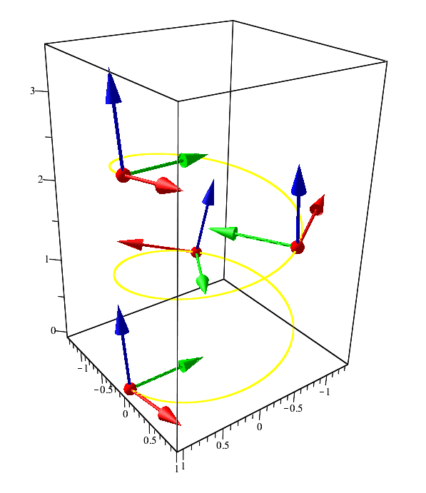
Curve "helix" and its vector: tangent - red, normal - green, binormal - blue



References:

Differential geometry of curves



If possible, to be continued ...