Aerobatic flight. Part 2. The simplest model of movement to perform the barrel
We continue a series of articles on the automation of the performance of pilotage figures on a small RPV. This article has, above all, an educational goal: here we will show how to create the simplest automatic control system (ACS) using the example of performing the “barrel” aerobatic operation while controlling an aircraft only with ailerons. The article is the second in the series of publications “Piloting RPV”, which tells about the process of building hardware and software parts of the ACS in a training form.

Link to the previous article of the cycle:
1. "Aerobatic flight. How to make a barrel "
Introduction
Movement model
Model parameters. Moment of inertia
Model parameters. Derivatives of moment roll
Model verification
Synthesis of control to perform the "barrel"
Flight experiment
Remarks
findings
So, we decided to implement the "barrel" in the automatic mode. It is obvious that for automatic execution of the figure it is necessary to formulate the corresponding control law. The process of inventing will be much more painless and faster if you use the mathematical model of the movement of the aircraft. Testing the control law in the flight experiment is possible, but it takes much longer, and it can be much more expensive in case of loss or damage to the vehicle.
Since at low angles of attack and gliding of the aircraft, its movement along the roll is practically unrelated to movement in two other channels: travel and longitudinal — to perform a simple “barrel” it will be enough to build a model of movement only around one axis, the OX axis of the associated SC . For the same reason, the aileron control law will not change significantly when it comes to creating a complete control system.
The equation of motion of the aircraft around the longitudinal axis OX of the connected SC is extremely simple:
Where - moment of inertia about axis OX , and moment consists of several components, of which for a realistic description of the movement of our aircraft, it is enough to consider only two:
Where - the moment caused by the rotation of the aircraft around the axis OX (damping moment), - the moment due to the deviation of the ailerons (control torque). The last expression is written in linearized form: roll moment linearly dependent on angular velocity and aileron deflection angle with constant coefficients of proportionality and respectively.
As is known (for example, from Wiki ), a linear differential equation
first order aperiodic link
Where - Transmission function, - differentiation operator, - time constant, and - gain.
For aperiodic link time constant equal to the time for which the output value with a single step effect of input value takes a value that differs from the steady state by ~ 5%, and the gain numerically equal to the steady-state value of the output value with a single step effect:

In the constructed motion model, there are two unknown parameters: the gain and time constant . These parameters are expressed through the characteristics of the physical system: moment of inertia , as well as the derivatives of the moment of roll and :
Thus, if the moment of inertia is known then, by defining the parameters of the model, it is possible to restore the system parameters from them.
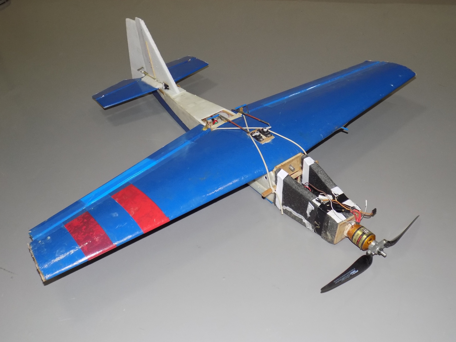
Our aircraft consists of the following parts: wing, fuselage with tail, engine, battery (battery) and avionics :

The avionics include: autopilot board, SNS receiver board, radio modem board, control signal receiver board, two voltage regulators, engine speed regulator, as well as connecting wires.

Due to the low weight of the avionics, its contribution to the total moment of inertia can be neglected.
The total value of the moment of inertia of the aircraft relative to the axis OX is obtained by adding the moments of inertia of the parts:
Assessing the contribution of each of the parts of the aircraft in the total moment of inertia , it turned out the following:
It is seen that the main contribution to the total moment of inertia makes the wing. This is due to the fact that the wing has a fairly large transverse size (wing span - 1 m):

Therefore, despite the modest weight (about 20% of the total take-off mass of the aircraft), the wing has a significant moment of inertia.
Calculation of the derivatives of the moment of roll is a rather difficult task associated with the calculation of the aerodynamic characteristics of the aircraft by numerical methods or using engineering techniques. The application of the first and second requires significant time, intellectual and computational costs, which are justified in the development of control systems for large aircraft, where the cost of the error still exceeds the cost of building a good model. For the task of controlling a UAV, whose mass does not exceed 2 kg, this approach is hardly justified. Another way to calculate these derivatives is flight experiment. Given the cheapness of our aircraft, as well as the proximity of a suitable field for such an experiment, the choice was obvious for us.
Writing into the autopilot firmware for manual control and registration of parameters, we assembled the plane and prepared it for testing:
In the flight experiment, it was possible to obtain data on the angle of deflection of the ailerons and the angular velocity of rotation of the aircraft. The pilot operated the aircraft in manual mode, performing flying in a circle, turning and "barrels", and the onboard equipment recorded and sent the necessary information to the ground station. As a result, the necessary dependencies were obtained: (degrees / s) and (b / r). Magnitude represents the normalized deflection angle of ailerons: the value 1 corresponds to the maximum deviation, and the value −1 to the minimum:

How now to determine and from the data? The answer is to measure the parameters of the transition process according to the graphs. and .
The result of determining the values of the time constant and the gain is as follows: , . These values of the coefficients at a known value of the moment of inertia The following values of the derivatives of the moment of roll correspond:
So, building a model, which is based on aperiodic link
it can be verified by inputting a signal obtained from the flight experiment, and compare the output signal of the model with the value , also obtained in the experiment.
The result of verification is shown in the figure:

As can be seen from the figure, the coincidence of the model with reality is slightly less than complete.
Having obtained the model, it is easy to determine by what amount and how long it is necessary to reject the ailerons in order to perform the “barrel”. One option is the following deviation algorithm:

The presence of segments with a duration of 0.1 s at the beginning and at the end of the aileron deflection algorithm models the inertia of the servo, which cannot deflect surfaces instantly. The model shows that with such a law, the deviations of the ailerons of the aircraft should perform one complete revolution around the axis OX , will we check?
The resulting aileron control law was programmed into the autopilot installed on the aircraft. The idea of the experiment is simple: bring the plane to horizontal flight, and then use the resulting control law. If the actual movement of the aircraft along the roll corresponds to the model created, the aircraft must perform a “barrel” - one full turn at 360 degrees.
Separately, we express our gratitude to our faithful pilot for his work, professionalism and comfortable trunk on the Priore-wagon!
In the course of the experiment, it became clear that the roll motion model was built successfully - the aircraft performed one “barrel” after another, as soon as the pilot activated the programmed control law. The following figure shows the angular velocity. recorded in the course of the experiment, and obtained from the simulation results, as well as the roll and pitch angle from the flight experiment:

The following figure shows the signals registered in the flight experiment on ailerons, elevator (RV) and rudder (PH):

The vertical lines indicate the beginning and end of the execution of the "barrel". From the figures it is clear that in the process of performing the “barrel” the pilot does not interfere with the control of the elevator and the rudder, it is also clear that the pitch angle invariably tends to decrease when performing the “barrel” - the plane delays into a dive, as predicted by the simulation results in the flight simulator (see the article "Aerobatic RPV. How to make a barrel" ). If you carefully review the previous graphs, it will become clear that the third “barrel” was not even finished, because the pilot intervened in the control to take the plane out of the dive: the pitch angle changes so much when performing “barrels” with ailerons alone.
As a result of the work we have done, we showed one of the ways to create a model of RPV motion by angular velocity. . In the flight experiment, it was proved that the created model of motion fully corresponds to the simulated object. On the basis of the developed model, the law of software control was obtained, which allows to perform the “barrel” in the automatic mode. We also made sure that it would not be possible to execute the correct “barrel” with the ailerons alone, and also demonstrated this clearly.
The next step will be the refinement of the control law by adding feedback, as well as the inclusion of the elevator in the control. The latter will require the creation of a model of the longitudinal movement of our aircraft. According to the results of the following publication.
Link to the previous article of the cycle:
1. "Aerobatic flight. How to make a barrel "
Content:
Introduction
Movement model
Model parameters. Moment of inertia
Model parameters. Derivatives of moment roll
Model verification
Synthesis of control to perform the "barrel"
Flight experiment
Remarks
findings
Introduction
So, we decided to implement the "barrel" in the automatic mode. It is obvious that for automatic execution of the figure it is necessary to formulate the corresponding control law. The process of inventing will be much more painless and faster if you use the mathematical model of the movement of the aircraft. Testing the control law in the flight experiment is possible, but it takes much longer, and it can be much more expensive in case of loss or damage to the vehicle.
Since at low angles of attack and gliding of the aircraft, its movement along the roll is practically unrelated to movement in two other channels: travel and longitudinal — to perform a simple “barrel” it will be enough to build a model of movement only around one axis, the OX axis of the associated SC . For the same reason, the aileron control law will not change significantly when it comes to creating a complete control system.
Movement model
The equation of motion of the aircraft around the longitudinal axis OX of the connected SC is extremely simple:
Where - moment of inertia about axis OX , and moment consists of several components, of which for a realistic description of the movement of our aircraft, it is enough to consider only two:
Where - the moment caused by the rotation of the aircraft around the axis OX (damping moment), - the moment due to the deviation of the ailerons (control torque). The last expression is written in linearized form: roll moment linearly dependent on angular velocity and aileron deflection angle with constant coefficients of proportionality and respectively.
As is known (for example, from Wiki ), a linear differential equation
first order aperiodic link
Where - Transmission function, - differentiation operator, - time constant, and - gain.
How to move from a differential equation to a transfer function?
In our case, from the parameters of the equation to the parameters of the transfer function, you can go as follows (knowing that the derivative negative):
For aperiodic link time constant equal to the time for which the output value with a single step effect of input value takes a value that differs from the steady state by ~ 5%, and the gain numerically equal to the steady-state value of the output value with a single step effect:
In the constructed motion model, there are two unknown parameters: the gain and time constant . These parameters are expressed through the characteristics of the physical system: moment of inertia , as well as the derivatives of the moment of roll and :
Thus, if the moment of inertia is known then, by defining the parameters of the model, it is possible to restore the system parameters from them.
Model parameters. Moment of inertia
Our aircraft consists of the following parts: wing, fuselage with tail, engine, battery (battery) and avionics :
The avionics include: autopilot board, SNS receiver board, radio modem board, control signal receiver board, two voltage regulators, engine speed regulator, as well as connecting wires.
Due to the low weight of the avionics, its contribution to the total moment of inertia can be neglected.
How was the estimation of the moment of inertia?
Estimation of the moment of inertia can be carried out as follows. Let's look at the plane along the axis OX :

And then we will present it in the form of the following simplified model:

Scheme for calculating the moment of inertia . Top left - the battery, bottom right - the engine. The engine and battery are located on the axis of the fuselage
It can be seen that for the creation of the model, the keel, horizontal tail, propeller and avionics were dropped. At the same time left: the fuselage, wing, battery, engine. By measuring the masses and characteristic dimensions of each part, it is possible to calculate the moments of inertia of each part relative to the longitudinal axis of the fuselage:
And then we will present it in the form of the following simplified model:
Scheme for calculating the moment of inertia . Top left - the battery, bottom right - the engine. The engine and battery are located on the axis of the fuselage
It can be seen that for the creation of the model, the keel, horizontal tail, propeller and avionics were dropped. At the same time left: the fuselage, wing, battery, engine. By measuring the masses and characteristic dimensions of each part, it is possible to calculate the moments of inertia of each part relative to the longitudinal axis of the fuselage:
- wing (thin rod):
- fuselage (hollow cylinder):
- battery (plate):
- engine (drive):
The total value of the moment of inertia of the aircraft relative to the axis OX is obtained by adding the moments of inertia of the parts:
Assessing the contribution of each of the parts of the aircraft in the total moment of inertia , it turned out the following:
- wing - 96.3%,
- fuselage - 1.6%,
- engine and battery - 2%,
It is seen that the main contribution to the total moment of inertia makes the wing. This is due to the fact that the wing has a fairly large transverse size (wing span - 1 m):
Therefore, despite the modest weight (about 20% of the total take-off mass of the aircraft), the wing has a significant moment of inertia.
Model parameters. Derivatives of moment roll and
Calculation of the derivatives of the moment of roll is a rather difficult task associated with the calculation of the aerodynamic characteristics of the aircraft by numerical methods or using engineering techniques. The application of the first and second requires significant time, intellectual and computational costs, which are justified in the development of control systems for large aircraft, where the cost of the error still exceeds the cost of building a good model. For the task of controlling a UAV, whose mass does not exceed 2 kg, this approach is hardly justified. Another way to calculate these derivatives is flight experiment. Given the cheapness of our aircraft, as well as the proximity of a suitable field for such an experiment, the choice was obvious for us.
Writing into the autopilot firmware for manual control and registration of parameters, we assembled the plane and prepared it for testing:
In the flight experiment, it was possible to obtain data on the angle of deflection of the ailerons and the angular velocity of rotation of the aircraft. The pilot operated the aircraft in manual mode, performing flying in a circle, turning and "barrels", and the onboard equipment recorded and sent the necessary information to the ground station. As a result, the necessary dependencies were obtained: (degrees / s) and (b / r). Magnitude represents the normalized deflection angle of ailerons: the value 1 corresponds to the maximum deviation, and the value −1 to the minimum:
How now to determine and from the data? The answer is to measure the parameters of the transition process according to the graphs. and .
How were the k and T coefficients determined?
Gain determined by assigning the magnitude of the steady-state value of the angular velocity to the deviation of the aileron:

The dependences of the deflection angle of ailerons and the angular velocity of the roll on time, obtained in the flight experiment
In the previous figure, the segments of the steady-state value of the angular velocity approximately correspond, for example, to the segments near the time points 422, 425, and 438 s (marked in dark red in the figure).
Time constant determined from the same graphs. For this, areas of abrupt change in the aileron deflection angle were found, and then the time was taken for which the angular velocity takes a value that differs from the steady-state value by 5%.
The result of determining the values of the time constant and the gain is as follows: , . These values of the coefficients at a known value of the moment of inertia The following values of the derivatives of the moment of roll correspond:
Model verification
So, building a model, which is based on aperiodic link
it can be verified by inputting a signal obtained from the flight experiment, and compare the output signal of the model with the value , also obtained in the experiment.
How was the simulation?
We chose a tool for modeling, first of all, based on the possibility of repetition of the results by a wide range of readers: this primarily means that the program should be publicly available. In principle, the problem of modeling the behavior of aperiodic link of the first order can be solved by creating your own tool from scratch. But since in the future the model will become more complex, the creation of its tool can distract from the main task - the creation of an ACS piloting RPV. Taking into account the principle of openness of the tool, we chose JSBsim .
In the previous section, we obtained the values of the coefficients and . We use them to simulate the movement of the aircraft. From the last article, we remember that the aircraft model configuration in JSBsim is specified using an XML file. Create your own model:
Since we are building a model of movement of the apparatus only on roll, we will leave many of the sections of the file empty. The following characteristics are sequentially set in the model file.
Geometric dimensions of the aircraft are set in the metrics section: wing area, span, average aerodynamic chord length, horizontal tail area, horizontal tail, vertical tail area, vertical tail, and aerodynamic focus position.
The mass characteristics of the aircraft are specified in the mass_balance section: the inertia tensor of the aircraft, the weight of the empty aircraft, the position of the center of mass.
It should be noted that the absolute positions of the aerodynamic focus and the center of mass of the aircraft do not participate in the calculation of the dynamics of the apparatus, their relative location is important.
This is followed by sections describing the characteristics of the chassis of the aircraft and its power plant.
In the next section responsible for the control system , fill the channel responsible for roll control: we specify the only input fcs / aileron-cmd-norm , the value of which will be normalized from -1 to 1.
Aerodynamic characteristics are set in the aerodynamics section: forces are set in the high-speed coordinate system, moments in the connected one. We are interested in the moment roll. In the section axis name = “ROLL”, functions are defined that determine the moment of forces from the various components of the projection of the moment of aerodynamic forces on the axis OX of the associated coordinate system. In our model there are two such components. The first component is the damping moment, which is equal to the product of the angular velocity by the previously determined coefficient . The second component is the moment from the ailerons at a fixed flight speed: it is equal to the product of the previously determined coefficient the amount of deviation of the aileron.
It is worth noting that when determining the ratio dimensional value was used . In our flight data, the angular velocity was measured in degrees per second, whereas in JSBSim radians per second are used, so the coefficient should be reduced to the dimension we need, that is, divided by 180 degrees and multiplied by radian. We write these components of the moment of aerodynamic forces inside the functions of the product product . In the simulation, the result of performing all the functions is summed up and the value of the projection of the aerodynamic moment on the corresponding axis is obtained.
The created model can be checked on the experimental data obtained during flight tests. To do this, create a script with the following content:
where dots indicate missing data. In the file of the script familiar to us from the previous article, a new type of event ( “Time Notif” ) has appeared, which allows setting a continuous parameter change over time. The dependence of the parameter on time is given by a table function. JSBSim linearly interpolates the value of a function between tabular data. The verification procedure of the roll motion model consists in the execution of this script on the created model and comparing the results with the experimental ones.
In the previous section, we obtained the values of the coefficients and . We use them to simulate the movement of the aircraft. From the last article, we remember that the aircraft model configuration in JSBsim is specified using an XML file. Create your own model:
<?xml version="1.0"?> <fdm_config name="OP1" version="2.0" release="BETA"> <metrics> <wingarea unit="M2"> 0.2 </wingarea> <wingspan unit="M"> 1.0 </wingspan> <chord unit="M"> 0.2 </chord> <htailarea unit="M2"> 0.03 </htailarea> <htailarm unit="M"> 0.5 </htailarm> <vtailarea unit="M2"> 0.03 </vtailarea> <vtailarm unit="M"> 0.5 </vtailarm> <location name="AERORP" unit="M"> <x> -0.025 </x> <y> 0 </y> <z> 0.05 </z> </location> </metrics> <mass_balance> <ixx unit="KG*M2"> 0.018 </ixx> <iyy unit="KG*M2"> 0.018 </iyy> <izz unit="KG*M2"> 0.018 </izz> <emptywt unit="KG"> 1.2 </emptywt> <location name="CG" unit="M"> <x> 0 </x> <y> 0 </y> <z> 0 </z> </location> </mass_balance> <ground_reactions> </ground_reactions> <propulsion> </propulsion> <flight_control name="FCS: OP1"> <channel name="Pitch"> </channel> <channel name="Roll"> <summer name="Roll Trim Sum"> <input>fcs/aileron-cmd-norm</input> <clipto> <min>-1</min> <max>1</max> </clipto> </summer> </channel> <channel name="Yaw"> </channel> </flight_control> <aerodynamics> <axis name="DRAG"> </axis> <axis name="SIDE"> </axis> <axis name="LIFT"> </axis> <axis name="ROLL" unit="N*M"> <function name="aero/coefficient/Clp"> <description>Roll_moment_due_to_roll_rate</description> <product> <property>velocities/p-aero-rad_sec</property> <value>-0.24</value> </product> </function> <function name="aero/coefficient/Clda"> <description>Roll_moment_due_to_aileron</description> <product> <property>fcs/aileron-cmd-norm</property> <value> 2.4 </value> </product> </function> </axis> <axis name="PITCH"> </axis> <axis name="YAW"> </axis> </aerodynamics> <output name="OP1.csv" rate="60" type="CSV"> <property> velocities/vc-kts </property> <property> aero/alphadot-deg_sec </property> <property> aero/betadot-deg_sec </property> <property> fcs/throttle-cmd-norm </property> <simulation> OFF </simulation> <atmosphere> OFF </atmosphere> <massprops> OFF </massprops> <aerosurfaces> ON </aerosurfaces> <rates> ON </rates> <velocities> ON </velocities> <forces> OFF </forces> <moments> OFF </moments> <position> ON </position> <coefficients> OFF </coefficients> <ground_reactions> OFF </ground_reactions> <fcs> ON </fcs> <propulsion> OFF </propulsion> </output> </fdm_config>
Since we are building a model of movement of the apparatus only on roll, we will leave many of the sections of the file empty. The following characteristics are sequentially set in the model file.
Geometric dimensions of the aircraft are set in the metrics section: wing area, span, average aerodynamic chord length, horizontal tail area, horizontal tail, vertical tail area, vertical tail, and aerodynamic focus position.
The mass characteristics of the aircraft are specified in the mass_balance section: the inertia tensor of the aircraft, the weight of the empty aircraft, the position of the center of mass.
It should be noted that the absolute positions of the aerodynamic focus and the center of mass of the aircraft do not participate in the calculation of the dynamics of the apparatus, their relative location is important.
This is followed by sections describing the characteristics of the chassis of the aircraft and its power plant.
In the next section responsible for the control system , fill the channel responsible for roll control: we specify the only input fcs / aileron-cmd-norm , the value of which will be normalized from -1 to 1.
Aerodynamic characteristics are set in the aerodynamics section: forces are set in the high-speed coordinate system, moments in the connected one. We are interested in the moment roll. In the section axis name = “ROLL”, functions are defined that determine the moment of forces from the various components of the projection of the moment of aerodynamic forces on the axis OX of the associated coordinate system. In our model there are two such components. The first component is the damping moment, which is equal to the product of the angular velocity by the previously determined coefficient . The second component is the moment from the ailerons at a fixed flight speed: it is equal to the product of the previously determined coefficient the amount of deviation of the aileron.
It is worth noting that when determining the ratio dimensional value was used . In our flight data, the angular velocity was measured in degrees per second, whereas in JSBSim radians per second are used, so the coefficient should be reduced to the dimension we need, that is, divided by 180 degrees and multiplied by radian. We write these components of the moment of aerodynamic forces inside the functions of the product product . In the simulation, the result of performing all the functions is summed up and the value of the projection of the aerodynamic moment on the corresponding axis is obtained.
The created model can be checked on the experimental data obtained during flight tests. To do this, create a script with the following content:
<?xml version="1.0" encoding="utf-8"?> <runscript> <use aircraft="ownPlane1" initialize="scripts/airborne"/> <run start="0" end="51" dt="0.01"> <event name="Trims"> <condition> sim-time-sec ge 0.0 </condition> <set name="simulation/do_simple_trim" value="5"/> </event> <event name="Time Notif" continuous="true"> <description>Provide a time history input for the aileron</description> <condition> sim-time-sec ge 0</condition> <set name="fcs/aileron-cmd-norm" > <function> <table> <independentVar lookup="row">sim-time-sec</independentVar> <tableData> 0 0.00075 0.1 0.00374 0.2 -0.00075 0.3 -0.00075 0.4 -0.00075 0.5 -0.00075 0.6 0.00075 0.7 0.00075 ... 48.8 -0.00075 48.9 0.00000 49 -0.00075 </tableData> </table> </function> </set> </event> </run> </runscript>
where dots indicate missing data. In the file of the script familiar to us from the previous article, a new type of event ( “Time Notif” ) has appeared, which allows setting a continuous parameter change over time. The dependence of the parameter on time is given by a table function. JSBSim linearly interpolates the value of a function between tabular data. The verification procedure of the roll motion model consists in the execution of this script on the created model and comparing the results with the experimental ones.
The result of verification is shown in the figure:
As can be seen from the figure, the coincidence of the model with reality is slightly less than complete.
Synthesis of control to perform the "barrel"
Having obtained the model, it is easy to determine by what amount and how long it is necessary to reject the ailerons in order to perform the “barrel”. One option is the following deviation algorithm:
- : ailerons begin to deviate from the neutral position;
- : ailerons rejected by 50%;
- : ailerons begin to deviate to the neutral position;
- : ailerons in neutral.
The presence of segments with a duration of 0.1 s at the beginning and at the end of the aileron deflection algorithm models the inertia of the servo, which cannot deflect surfaces instantly. The model shows that with such a law, the deviations of the ailerons of the aircraft should perform one complete revolution around the axis OX , will we check?
Flight experiment
The resulting aileron control law was programmed into the autopilot installed on the aircraft. The idea of the experiment is simple: bring the plane to horizontal flight, and then use the resulting control law. If the actual movement of the aircraft along the roll corresponds to the model created, the aircraft must perform a “barrel” - one full turn at 360 degrees.
Separately, we express our gratitude to our faithful pilot for his work, professionalism and comfortable trunk on the Priore-wagon!
In the course of the experiment, it became clear that the roll motion model was built successfully - the aircraft performed one “barrel” after another, as soon as the pilot activated the programmed control law. The following figure shows the angular velocity. recorded in the course of the experiment, and obtained from the simulation results, as well as the roll and pitch angle from the flight experiment:
The following figure shows the signals registered in the flight experiment on ailerons, elevator (RV) and rudder (PH):
The vertical lines indicate the beginning and end of the execution of the "barrel". From the figures it is clear that in the process of performing the “barrel” the pilot does not interfere with the control of the elevator and the rudder, it is also clear that the pitch angle invariably tends to decrease when performing the “barrel” - the plane delays into a dive, as predicted by the simulation results in the flight simulator (see the article "Aerobatic RPV. How to make a barrel" ). If you carefully review the previous graphs, it will become clear that the third “barrel” was not even finished, because the pilot intervened in the control to take the plane out of the dive: the pitch angle changes so much when performing “barrels” with ailerons alone.
Remarks
- Built ACS to perform the "barrel" does not take into account the dependence of the derivatives of the moment of the roll on the flight speed. On the one hand, this was done in order not to complicate the model and the law of control. On the other hand, such a dependence is easy to introduce if instead of derivatives and use values and determined at a given flight speed .
- The developed control law is a program control without feedback. The presence of feedback on the angular velocity and / or roll angle will improve the accuracy of the figure, which will be done in the future.
findings
As a result of the work we have done, we showed one of the ways to create a model of RPV motion by angular velocity. . In the flight experiment, it was proved that the created model of motion fully corresponds to the simulated object. On the basis of the developed model, the law of software control was obtained, which allows to perform the “barrel” in the automatic mode. We also made sure that it would not be possible to execute the correct “barrel” with the ailerons alone, and also demonstrated this clearly.
The next step will be the refinement of the control law by adding feedback, as well as the inclusion of the elevator in the control. The latter will require the creation of a model of the longitudinal movement of our aircraft. According to the results of the following publication.
All Articles