Station for measuring wind speed and direction
The usual household branded or self-made weather station measures two temperature-humidity (in the room and outside), atmospheric pressure, and additionally has a clock with a calendar. However, this meteorological station still has a lot of things - a solar radiation sensor, a precipitation meter and all that, which, in general, is required only for professional needs, with one exception. Measuring parameters of wind (speed, and, most importantly, the direction) - a very useful addition to a country house. Moreover, branded wind sensors are quite expensive even on Ali Baba, and it makes sense to look at homemade solutions.
I must say right away that if I knew in advance what amount of manual work and money spent on experiments my idea would flow, maybe I would not begin. But curiosity outweighed, and the readers of this article have a chance to avoid those pitfalls that I had to stumble over.
To measure wind speed (anemometry), there are stopitsot methods, the main of which are:
- thermo-anemometric,
- mechanical - with a propeller (more precisely, an impeller ) or a pan -shaped horizontal impeller (a classic pan-type anemometer ). Measuring the speed in these cases is equivalent to measuring the rotational speed of the axis on which the propeller or impeller is attached.
- as well as ultrasonic, combining measurements of speed and direction.
To measure the direction of the methods less:
- mentioned ultrasound;
- mechanical vane with electronic removal of the angle of rotation. There are also many different ways to measure the angle of rotation: optical, resistive, magnetic, inductive, mechanical. You can, by the way, just fix an electronic compass on the shaft of the weather vane - only reliable and simple (for “knee-like” repetition) methods of transferring readings from a randomly rotating axis will have to be searched. Therefore, we further choose the traditional optical method.
When self-repeating any of these methods, one should keep in mind the requirements of minimum energy consumption and round-the-clock (and maybe year-round?) Stay in the sun and in the rain. The wind sensor cannot be placed under the roof in the shade - on the contrary, it should be as far as possible from all interfering factors and “open to all winds”. The ideal location is the ridge of the house or, at worst, the shed or arbours, remote from other buildings and trees. Such requirements assume autonomous power and, obviously, a wireless data transmission channel. These requirements are due to some "bells and whistles" of the design, which is described below.
The cognitive story of how I tried to reproduce the most modern and advanced of the ways - ultrasound, and failed, I will tell you some other time. All other methods involve a separate measurement of speed and direction, so I had to fence two sensors. Having learned the thermoanemometers theoretically, I realized that the ready-made sensitive element of the amateur level could not be obtained from us (they are available on the western market!), And to independently get involved in the next R & D with the corresponding time and money wasted. Therefore, by some reflection, I decided to make a unified design for both sensors: a cup anemometer with optical measurement of rotational speed and a weather vane with an electronic rotation angle reading based on a coding disk (encoder).
The advantage of mechanical sensors is that no R & D is required there, the principle is simple and straightforward, and the quality of the result depends only on the accuracy of execution of a carefully thought-out design.
It seemed so theoretically, in practice, this resulted in a bunch of mechanical work, some of which had to be ordered on the side, due to the lack of turning and milling machines at hand. I must say at once that I have never regretted that from the very beginning I relied on the capital approach, and did not begin to fence designs from scrap materials.
For the wind vane and anemometer, the following parts are needed, which had to be ordered from the turner and miller (the quantity and material are indicated for both sensors at once):
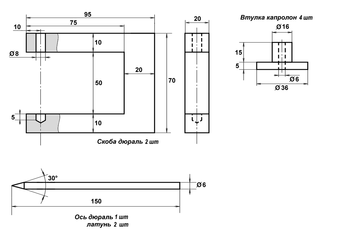
We note that axes are necessarily machined on a lathe: it is almost impossible to make an axle with a point exactly in the center on the knee. And the placement of the tip exactly along the axis of rotation here is the determining factor for success. In addition, the axis should be perfectly straight, no deviations are allowed.
The basis of the wind vane (as well as the speed sensor below) is the U-shaped bracket made of D-16 duralumin, shown in the drawing at the top left. A piece of PTFE is pressed into the lower recess, in which a step recess is made in succession with 2 and 3 mm drills. An axle is inserted into this recess with a sharp end (brass for the weather vane). From above, it passes freely through an 8 mm hole. Over this hole with screws M2, a rectangular piece of the same fluoroplastic 4 mm thick is attached to the bracket so that it overlaps the hole. In PTFE, a hole is made exactly along the axis diameter of 6 mm (located exactly along the common axis of the holes - see the assembly drawing below). Fluoroplastic at the top and bottom here plays the role of sliding bearings.
The axis in the place of friction on the fluoroplast can be polished, and the area of friction can be reduced by rebounding a hole in the fluoroplastic. ( See on this topic below UPD from 09/13/18 ). For the weather vane, this does not play a special role - some “inhibition” is even useful to him, and for the anemometer you will have to try to minimize friction and inertia.
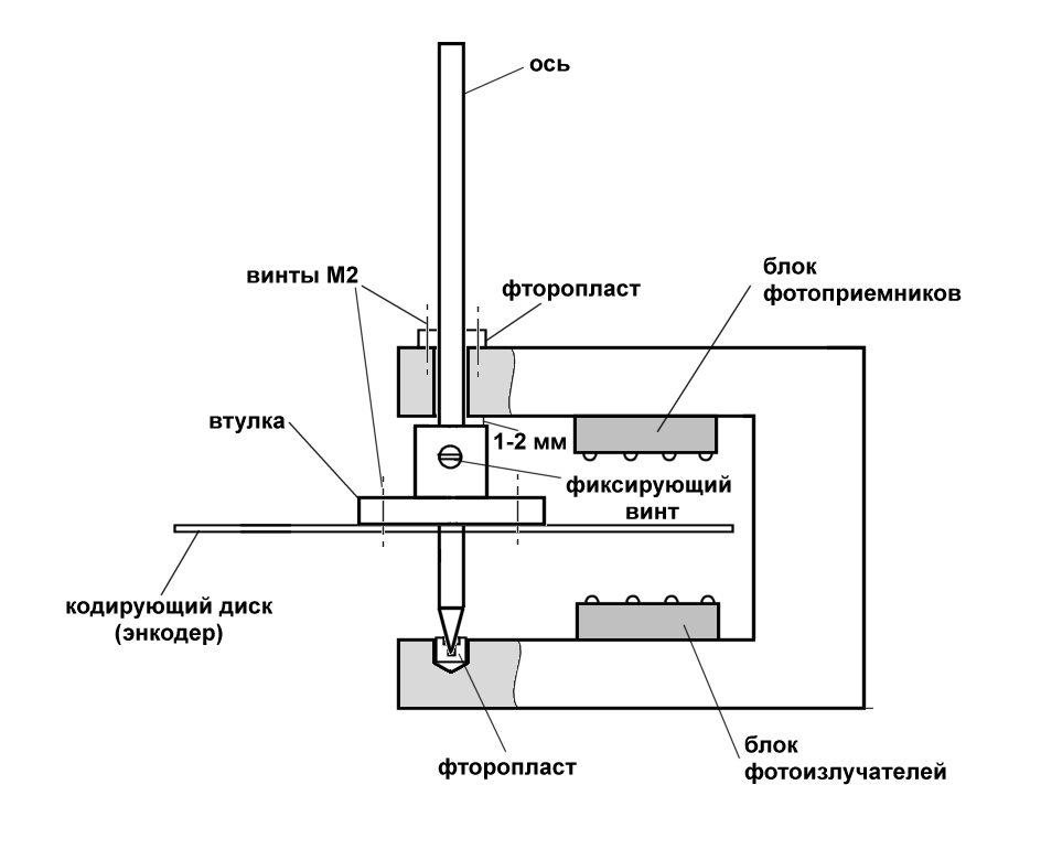
Now about the removal of the angle of rotation. Gray's classic encoder with 16 positions applied to our case looks as shown in the figure:

The disk size was chosen based on the condition of reliable optical isolation of the emitter-receiver pairs from each other. With this configuration, the slots 5 mm wide are also spaced 5 mm apart, and the optical pairs are located at a distance of exactly 10 mm. The dimensions of the bracket to which the vane is attached were calculated precisely on the basis of a disk diameter of 120 mm. All this, of course, can be reduced (especially if the LEDs and photodetectors are selected as small as possible), but the complexity of manufacturing the encoder was taken into account: it turned out that millers do not undertake such delicate work, because it had to be cut out manually with a file. And then the larger the size, the more reliable the result and less trouble.
The assembly drawing above shows the mounting of the disc to the axis. A carefully centered disc is attached to the caprolon hub with M2 screws. The sleeve is placed on the axis so that the gap at the top is minimal (1-2 mm) - so that the axis rotates freely in its normal position, and the tip does not fall out of the slot at the bottom when flipping. The blocks of photodetectors and emitters are attached to the bracket above and below the disk, more specifically about their design further.
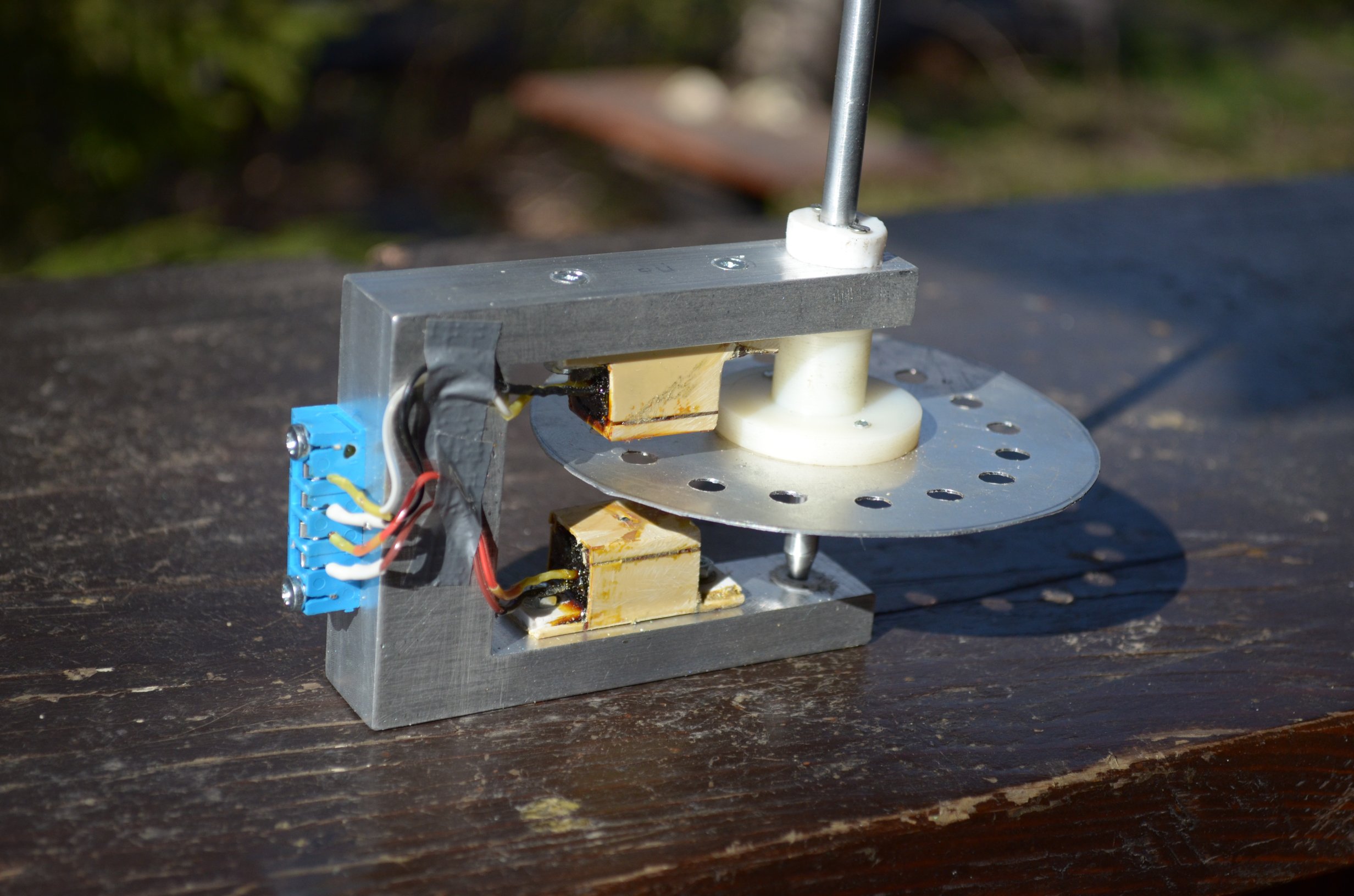
The whole structure is placed in a plastic (ABS or polycarbonate) case 150 × 150 × 90 mm. In assembled form (without a cover and a weather vane), the direction sensor looks as follows:
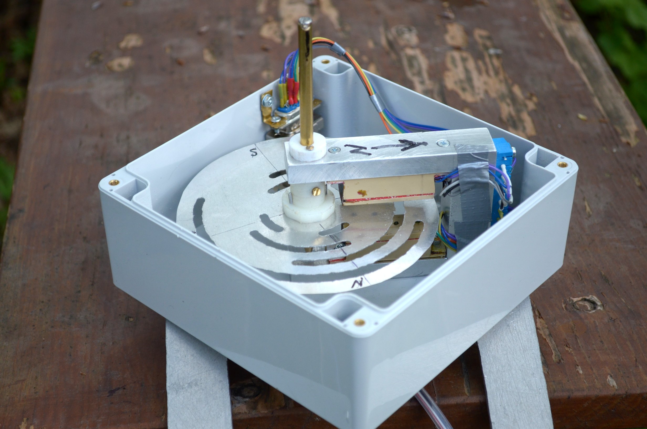
Note that the selected direction to the north is marked with an arrow; it will need to be observed when installing the sensor in place.
At the top of the axis is attached to the actual vane. It is made on the basis of the same brass axis, in the incision on the blunt side of which the shank of brass sheet is soldered. At the sharp end, the thread M6 is cut at a certain length, and a round load-counterweight cast from lead is fixed on it with the help of nuts:
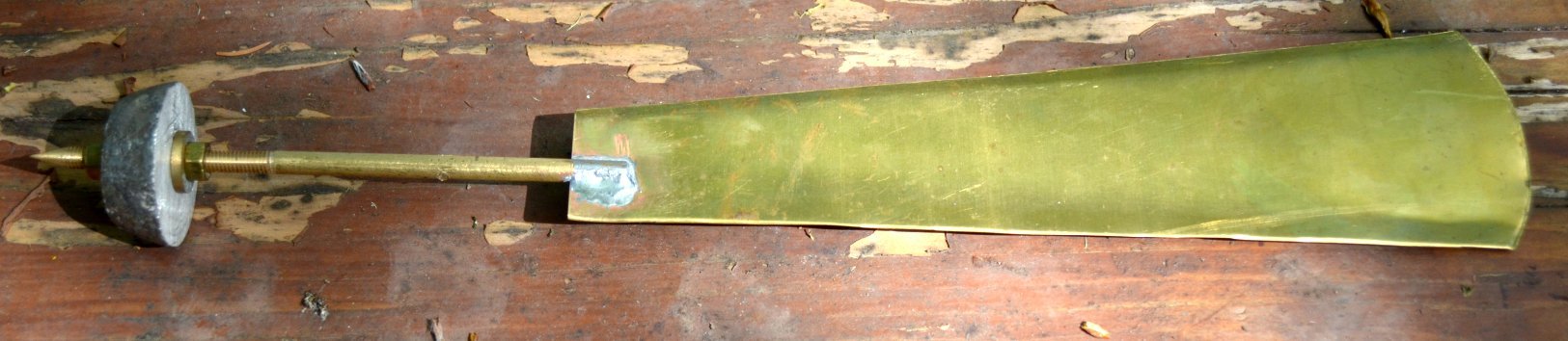
The load is designed so that the center of gravity falls exactly on the attachment point (by moving it along the thread, you can achieve perfect balancing). The wind vane is fixed to the axis by means of a stainless screw M3, which passes through a hole in the axis of the wind vane and is screwed into the thread cut into the axis of rotation (the fastening screw is visible in the photo above). For precise orientation, the top of the axis of rotation has a semicircular recess into which the axis of the vane lies.
As you already understood, the basis for the speed sensor for unification was chosen the same as for the weather vane. But the design requirements here are somewhat different: in order to reduce the starting point, the anemometer should be as light as possible. Therefore, in particular, the axis for it is made of duralumin, the disk with holes (for measuring the rotational speed) is reduced in diameter:
If four optocouplers are needed for a four-bit Gray encoder, there is only one for a speed sensor. 16 holes are drilled along the disk circumference at an equal distance; thus, one revolution of a disk per second is equivalent to 16 Hz of the frequency coming from the optocoupler (more openings are possible, smaller ones are possible - the question is only in the scale of recalculation and energy saving for radiators).
A home-made sensor will still be quite rough (the threshold of pulling away is at least half a meter-meter per second), but it can be lowered only if the design is radically changed: for example, you can install a propeller instead of a bowl turntable. In a bowl turntable, the difference in resistance to flow, which causes the torque, is relatively small - it is achieved solely due to the different shape of the surface meeting the incoming air flow (therefore the shape of the cups should be as streamlined as possible - ideally, it is half an egg or a ball). The propeller torque is much more, it can be made much smaller in weight, and, finally, the manufacture itself is simpler. But the propeller must be installed in the direction of air flow - for example, placing it on the end of the same weather vane .
The question of questions is: how to transfer readings from a sensor that randomly rotates around a vertical axis? I could not solve it, and judging by the fact that professional cup designs are still widespread, it is decided not to take a half-kick (manual anemometers are not taken into account - they are oriented manually by the air flow).
My version of the cup anemometer is made on the basis of a laser disk. Top and bottom view shown in the photo:
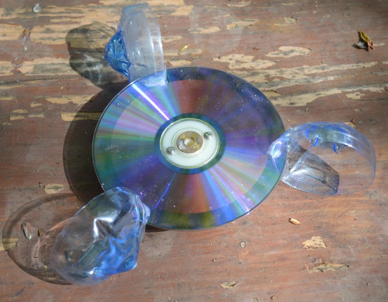
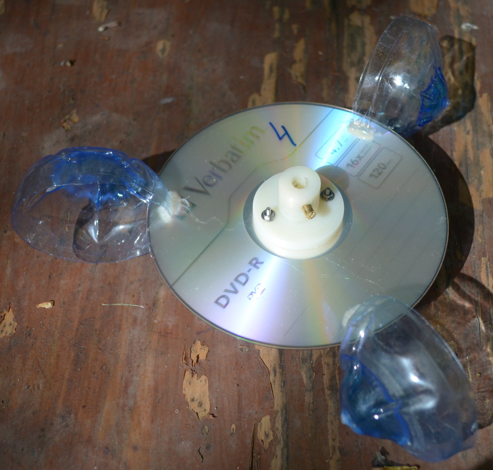
The cups are made of bottoms from bottles from under the Agusha water for children. The bottom is carefully cut off, and all three at the same distance so that they have equal weight, locally heated in the center (in any case, do not heat it completely - it will irreversibly twist!) And with the back of the wooden handle from the file it bends outwards to make it more streamlined. You will repeat - stock up with more bottles, from five to six pieces you will probably be able to make three more or less identical cups. In the manufactured cups, a slot is made on the side and they are fixed along the disc perimeter under 120 ° with respect to each other with the help of waterproof glue-sealant. The disk is strictly centered relative to the axis (I did this with the help of a nested metal washer) and fixed to the caprolon bushing with M2 screws.
Both sensors, as already mentioned, are placed in plastic housings 150 × 150 × 90 mm. It is necessary to approach the choice of material of the case thoughtfully: ABS or polycarbonate have sufficient weather resistance, but polystyrene, plexiglas and especially polyethylene will definitely not work here (and it will be difficult to paint them for sun protection too). If it is not possible to purchase a branded box, it is better to solder the body of foil-clad fiberglass laminate on its own, and then paint it for corrosion protection and aesthetic appearance.
In the lid, exactly in the place of the axis exit, a hole of 8-10 mm is made, into which the plastic cone cut from the spout from the spray can with construction sealant or glue is glued in with the same adhesive-sealant:
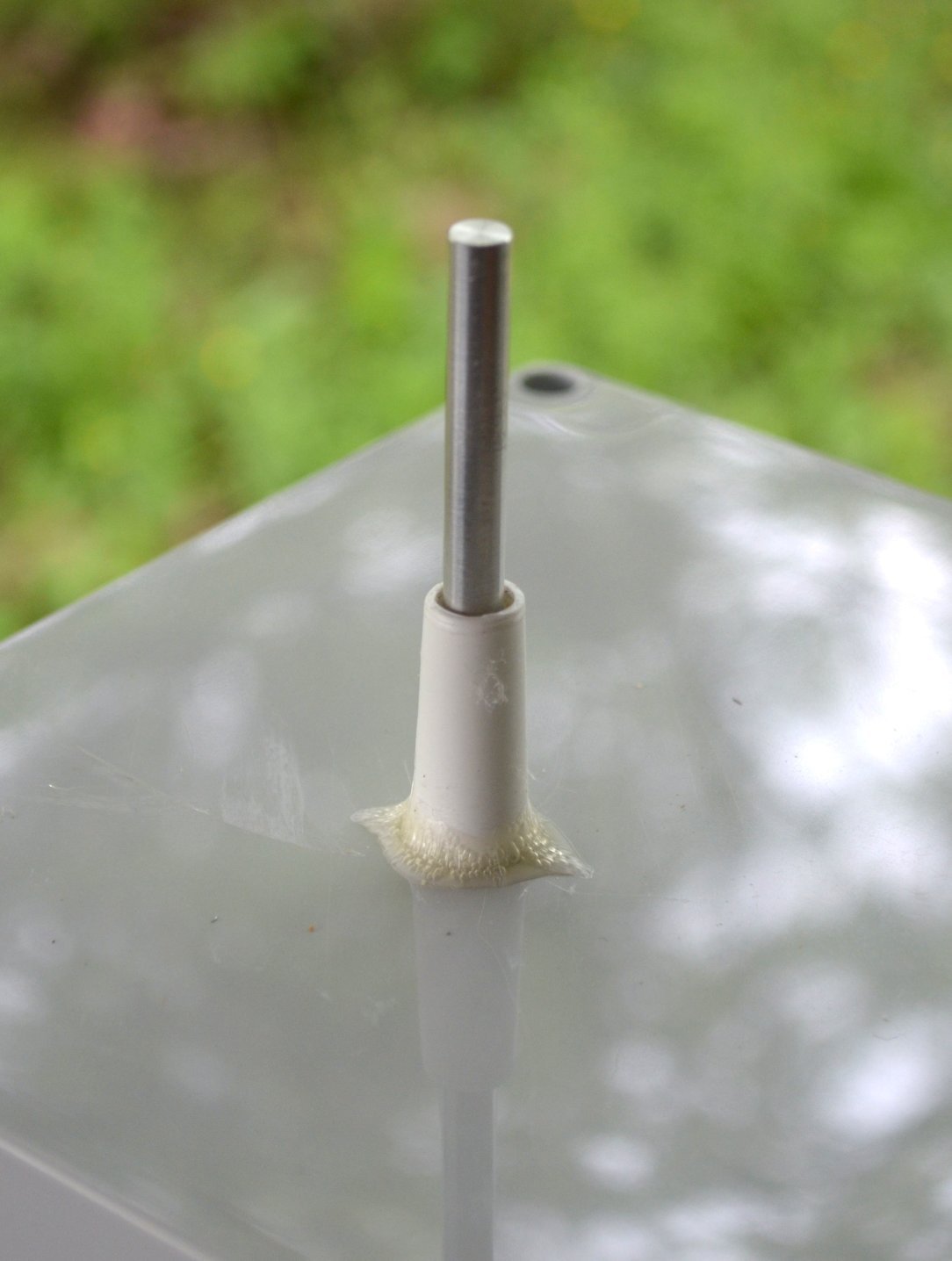
To center the cone axially, with a clamp, fasten a piece of wood from the bottom of the lid, mark the exact center on it and dive a little with a 12 mm perforated drill, making an annular recess around the hole. The cone has to enter there exactly, after which it can be coated with glue. You can additionally fix it in a vertical position for the time it hardens with an M6 screw and a nut.
The speed sensor itself covers the axis with this cone, like an umbrella, preventing water from entering the body. For a weather vane, it is worthwhile to additionally place a sleeve above the cone, which will close the gap between the axis and the cone from direct water flow (see the photo of the general view of the sensors below).
I have the wires from the optocouplers connected to a separate D-SUB connector (see photo of the direction sensor above). The mate with the cable is inserted through a rectangular hole in the base of the housing. The hole is then covered with a cover with a slot for the cable that keeps the connector from falling out. Duralumin brackets are screwed to the base of the case for fastening in place. Their configuration depends on the location of the sensors.
When assembled, both sensors look like this:
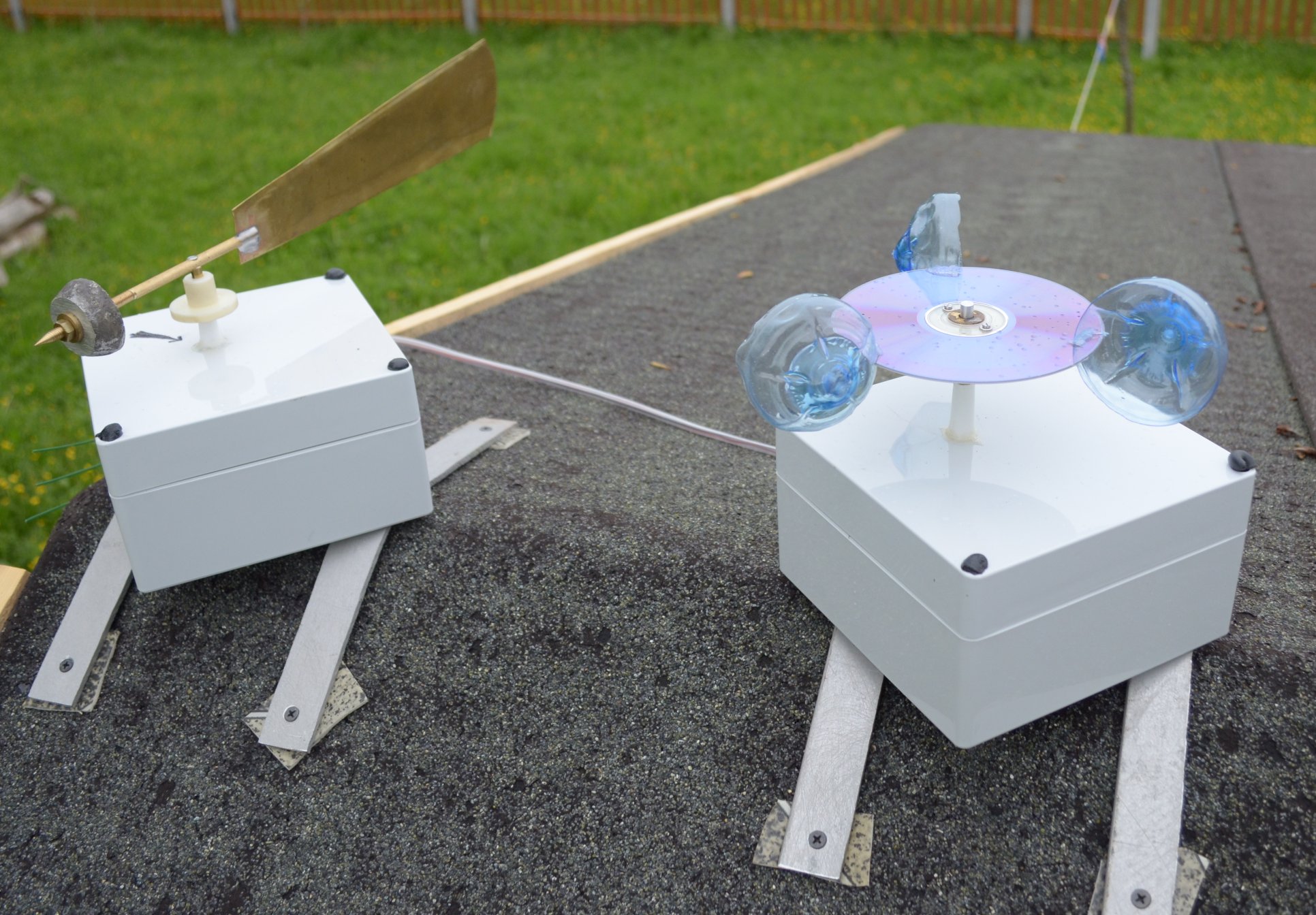
Here they are shown already installed in place - on the ridge of the arbor. Please note that the recesses for securing the cover screws are protected from water by raw rubber plugs. The sensors are installed horizontally in a horizontally level, for which they had to use linings made from pieces of linoleum.
The weather station as a whole consists of two modules: a remote unit (which serves both wind sensors and also reads from an external temperature-humidity sensor), and a main module with displays. The remote unit is equipped with a wireless transmitter for sending data installed inside it (the antenna sticks out from the side). The main module receives data from the remote unit (for convenience of its orientation, the receiver is placed on the cable in a separate unit), and also takes readings from the internal temperature-humidity sensor and displays all this on the displays. A separate component of the main unit is a clock with a calendar, which, for the convenience of the overall setup of the station, is serviced by a separate Arduino Mini controller, and have their own displays.
The photo emitters were chosen to use the infrared LEDs of the AL-107B. These vintage LEDs, of course, are not the best in their class, but they have a miniature case with a diameter of 2.4 mm and are capable of transmitting current up to 600 mA per pulse. By the way, during tests it turned out that the sample of this LED around 1980 release (in the red case) has about twice the efficiency (expressed in the range of confident photodetector operation) than modern specimens purchased in Chip-Dip (they have a transparent yellowish-green body). It is unlikely that in 1980 the crystals were better than now, although what the hell is not joking? Perhaps, however, the matter is in different scattering angles in both designations.
A constant current of about 20 mA (150 ohm resistor with 5 volt power supply) was passed through the LED in the speed sensor, and a pulse current (meander with a duty cycle of 2) current of about 65 mA (the same 150 ohm with 12 volt power) was passed in the direction sensor. The average current through one directional sensor LED is about 33 mA, in just four channels - about 130 mA.
As photodetectors, L-32P3C phototransistors in a case with a diameter of 3 mm were selected. The signal was filmed from a collector loaded on a 1.5 or 2 kΩ resistor from a 5 V power supply. These parameters are chosen so that at a distance of ~ 20 mm between the photo emitter and receiver, the controller input immediately receives a full-sized logic signal at 5-volt levels without additional amplification . The currents appearing here may seem disproportionately large if we proceed from the above stated minimum power consumption requirement, but as you will see, they appear in each measurement cycle for a maximum of a few milliseconds so that the total consumption remains small.
The basis for mounting the receivers and emitters served as segments of the cable channel (visible in the photo of the sensors above), cut so that at the base to form "ears" for mounting on the bracket. For each of these scraps a plastic plate was glued to the locking lid from the inside, the width equal to the width of the channel. The LEDs and phototransistors were fixed at the desired distance in the holes drilled in this plate so that the findings were inside the channel, and only the bulges on the end of the cases protruded. The pins are soldered in accordance with the scheme (see below), the external pins are made with flexible multi-colored wire cuts. Resistors for the direction sensor emitters are also located inside the channel, one common conclusion is made from them. After desoldering the lid snaps into place, all the cracks are sealed with clay and additionally with adhesive tape, which also closes the hole on the side opposite to the terminals, and the whole structure is filled with epoxy resin. External pins, as can be seen in the photo sensor, are displayed on the terminal block, mounted on the back side of the bracket.
The schematic diagram of the wind sensor processing unit is as follows:
About where the power is taken 12-14 volts, see below. In addition to the components indicated in the diagram, the remote unit contains a temperature-humidity sensor, which is not shown in the diagram. A voltage divider connected to pin A0 of the controller is designed to control the voltage of the power supply for the purpose of timely replacement. The LED connected to the traditional pin 13 (pin 19 of the DIP housing) is superbright, for its normal, non-glare glow, there is enough current in the milliampere fraction, which is ensured by the unusually high 33 kΩ resistor rating.
The scheme uses a “bare” Atmega328 controller in a DIP package, programmed via Uno and mounted on the panel. Such controllers with an Arduino downloader already recorded are sold, for example, in Chip-Dipe (or the downloader can be recorded independently ). Such a controller is convenient to program in a familiar environment, but, devoid of components on the board, it is, firstly, more economical, and secondly, it takes up less space. A full-fledged energy-saving mode could be obtained by getting rid of the bootloader too (and generally writing all the code in assembler :), but here it is not very relevant, and programming is unnecessarily complicated.
In the diagram, gray rectangles are circled with components related separately to the speed and direction channels. Consider the operation of the circuit as a whole.
The operation of the controller as a whole is controlled by the WDT watchdog timer enabled in the interrupt call mode. WDT takes the controller out of sleep at specified intervals. In case the timer is re-started in the called interrupt, the reset from scratch does not occur, all global variables remain at their values. This allows you to accumulate data from awakening to awakening and at some point to process them - for example, average.
At the beginning of the program, the following declarations of libraries and global variables are made (in order not to clutter the text of the already extensive examples, everything related to the temperature-humidity sensor is released here):
To initiate sleep and WDT (wake up every 4 seconds), use the following procedures:
The speed sensor outputs the frequency of interruption of the optical channel, the order of magnitude - units-tens of hertz. To measure such a value more economically and faster through the period (this was the subject of the publication of the author “ Evaluation of methods for measuring low frequencies on the Arduino ”). Here, the method is selected through the modified pulseInLong () function, which does not bind the measurement to specific controller outputs (the text of the periodInLong () function can be found in the specified publication).
The setup () function declares the directions of the outputs, initializes the 433 MHz transmitter library and the watchdog timer (the IN_PINF line is, in principle, superfluous, and inserted for the memory):
Finally, in the main program loop, we first, every time we wake up (every 4 seconds), read the voltage and calculate the frequency of the wind speed sensor:
The burning time of the IR LED (consuming, recall, 20 mA) here, as you can see, will be maximum if there is no rotation of the sensor disk and, under this condition, is about 0.25 seconds. The minimum measured frequency, therefore, will be 4 Hz (a quarter of a disk revolution per second with 16 holes). As it turned out when calibrating the sensor (see below), this corresponds to approximately 0.2 m / s wind speed. We emphasize that this is the minimum measured value of the wind speed, but not the resolution and not the starting point (which will be much higher). If there is a frequency (that is, when the sensor rotates), the measurement time (and, accordingly, the LED burning time, that is, the current consumption) will decrease proportionally, and the resolution will increase.
This is followed by the procedures that are performed every fourth awakening (that is, every 16 seconds). The value of the frequency of the speed sensor of the accumulated four values, we pass not the average, but the maximum - as experience has shown, this is a more informative value. Each of the values, regardless of its type, for convenience and uniformity, we turn into a positive integer with a size of 4 decimal places before transmission. The count variable keeps track of the number of awakenings:
Next is the definition of the Gray direction code. Here, to reduce consumption, instead of the permanently on IR LEDs, all four channels are simultaneously fed through the key field-effect transistor using the tone () function and a frequency of 5 kHz is applied. Detection of the presence of frequency on each of the digits (in_0p - in_3p pins) is made by the method similar to the anti-rattle when reading the pressed button. First, we wait in the loop if there is a high level at the output, and then check it after 100 μs. 100 μs is a half-frequency of 5 kHz, that is, if there is a frequency at least the second time, we will again get to a high level (we repeat four times just in case) and this means that it is exactly there. We repeat this procedure for each of the four bits of the code:
The maximum duration of one procedure will be in the absence of frequency at the receiver and is equal to 4 × 100 = 400 microseconds. The maximum burning time of 4 direction LEDs will be when no receiver is illuminated, that is, 4 × 400 = 1.6 milliseconds. The algorithm, by the way, will work in the same way if, instead of the frequency, the period of which is a multiple of 100 µs, just submit a constant high level to the LEDs. In the presence of a meander instead of a constant level, we simply save food by half. We can save even more if we get each IR LED through a separate line (respectively, through a separate controller output with its own key transistor), but this also complicates the circuit, wiring and control, and the current is 130 mA for 2 ms every 16 seconds - this is, you see, a little.
Finally, wireless data transmission . To transfer data from the sensor installation site to the weather station display, the simplest, cheapest and most reliable method was chosen: a transmitter / receiver pair at a frequency of 433 MHz . I agree that the method is not the most convenient (due to the fact that the devices are designed to transfer bit sequences, rather than whole bytes, you have to refine your data conversion between the necessary formats), and I am sure that many will want to argue with me in terms of its reliability. The answer to the last objection is simple: “you just do not know how to cook them!”.
The secret is that it usually remains beyond the frame of various descriptions of data exchange over the 433 MHz channel: since these devices are purely analog, the receiver power must be very well cleaned of any extraneous pulsations. In no case should not power the receiver from the internal 5-volt Arduino stabilizer! Installation for the receiver of a separate low-power stabilizer (LM2931, LM2950 or similar) directly in the vicinity of its findings, with the correct filtering circuits at the input and output, dramatically increases the range and reliability of transmission.
In this case, the transmitter worked directly from the battery voltage of 12 V, the receiver and the transmitter were equipped with standard homemade antennas in the form of a 17 cm long wire. (Let me remind you that the antenna wire is only single-core, and the antennas should be placed in space parallel to each other.) A packet of information of 24 bytes in length (taking into account humidity and temperature) without any problems was confidently transmitted at a speed of 1200 bps diagonally across the 15 hectare garden plot (about 40-50 meters), and then after three logs walls inside the room (in which, for example, the cellular signal is received with great difficulty and not everywhere). Conditions practically unattainable for any standard 2.4 GHz method (such as Bluetooth, Zig-Bee, and even amateur Wi-Fi), while the transmitter consumption here is a measly 8 mA and only at the moment of transmission, the rest of the time the transmitter consumes penny. The transmitter is structurally placed inside the remote unit, the antenna sticks out laterally horizontally.
We combine all the data into one packet (in a real station, temperature and humidity will be added to it), consisting of uniform 4-byte parts and preceded by the “DAT” signature, send it to the transmitter and complete all the cycles:
The packet size can be reduced if the requirement to represent each of the values of various types in the form of a uniform 4-byte code is refused (for example, one byte is enough for the Gray code, of course). But for the sake of universalization, I left everything as it is.
Power and design features of the remote unit . The consumption of the remote unit is calculated as follows:
- 20 mA (emitter) + ~ 20 mA (controller with auxiliary circuits) for about 0.25 every four seconds - on average 40/16 = 2.5 mA;
- 130 mA (emitters) + ~ 20 mA (controller with auxiliary circuits) for about 2 ms every 16 seconds - an average of 150/16/50 ≈ 0.2 mA;
Drawing on this calculation, the consumption of the controller when removing data from the temperature-humidity sensor and when the transmitter is working, we can safely bring the average consumption to 4 mA (at a peak of about 150 mA, notice!). The batteries (which, by the way, will require as many as 8 pieces to provide the transmitter with the maximum voltage!) Will have to be changed too often, because the idea arose of supplying the remote unit with 12-volt batteries for the screwdriver - I just got two of them superfluous. Their capacity is even less than the corresponding number of AA batteries - only 1.3 A • hours, but no one bothers to change them at any time, keeping the second charged at the ready. With the indicated consumption of 4 mA, the capacity of 1300 mA • hours is enough for about two weeks, which is not too troublesome.
Note that the voltage of a freshly charged battery can be up to 14 volts. In this case, an input stabilizer of 12 volts is installed - in order to prevent overvoltages of the transmitter power supply and not to overload the main five-volt stabilizer.
The remote unit in a suitable plastic case is placed under the roof, to it on the connectors summed up the power cable from the battery and the connection to the wind sensors. The main difficulty is that the circuit turned out to be extremely sensitive to the humidity of the air: in rainy weather, after a couple of hours, the transmitter begins to fail, the frequency measurements show a complete mess, and the battery voltage measurements show the “weather on Mars”.
Therefore, after debugging the algorithms and checking all the connections, the housing must be carefully sealed. All connectors at the entrance to the housing are coated with a sealant, the same applies to all screw heads protruding to the outside, the antenna output and the power cable. The joints of the case are plastered with plasticine (taking into account the fact that they will have to be separated), and additionally are glued on top with strips of sanitary tape. It is not bad to additionally strengthen the used connectors inside with epoxy: for example, the DB-15 module shown on the diagram of the external module is not sealed by itself, and moist air will slowly seep between the metal frame and the plastic base.
But all these measures by themselves will only give a short-term effect - even if there is no cold humid air suction, the dry air from the room easily turns into wet when the temperature outside the case falls (think of a phenomenon called “dew point”).
To avoid this, it is necessary to leave the cartridge or bag with a desiccant - silica gel inside the case (bags with it are sometimes put in boxes with shoes or in some packages with electronic devices). If the silica gel is of unknown origin and has been stored for a long time, it must be calcined in an electric oven at 140-150 degrees for several hours before use. If the case is sealed properly, then the desiccant will have to be changed no more than at the beginning of each summer season.
In the main module, all values are accepted, decoded, if necessary, converted in accordance with the calibration equations and displayed on the display.
The receiver is located outside the main module of the station and placed in a small box with ears for mounting. The antenna is brought out through the hole in the cover, all the holes in the body are sealed with wet rubber. The contacts of the receiver are brought to a very reliable domestic PC-4 type connector, from the receiver side it is connected through a piece of shielded dual AV cable:
A signal is picked up along one of the cable cores, the other is supplied with raw 9 volts from the module power adapter. The stabilizer type LM-2950-5.0 with filtering capacitors installed in a box with the receiver on a separate scarf.
Experiments were carried out to increase the length of the cable (just in case - suddenly it wouldn't work through the wall?), In which it turned out that nothing changes within the limits of length up to 6 meters.
There are only four OLED displays: two yellow serve weather data, two green clocks and a calendar. Their placement is shown in the photo:
Please note that in each group one of the displays is text, the second is graphic, with artificially created fonts in the form of glyph pictures. Here we will not dwell on the issue of displaying information on displays in order not to inflate the already extensive text of the article and examples: due to the presence of glyph pictures that have to be output individually (often simply by enumerating options by the case statement), output programs can be very cumbersome. For information on how to handle such displays, see the author’s publication Graphic and Text Mode of Winstar Displays , including an example of a display for displaying wind data.
Schematic diagram. For convenience, the clocks and their displays are serviced by a separate Arduino Mini controller and we will not analyze them anymore. The scheme of connecting components to Arduino Nano, which controls the reception and output of weather data, is as follows:
Here, unlike the remote module, the connection of weather sensors - a barometer and an internal temperature-humidity sensor is shown. Attention should be paid to the power wiring - the displays are powered by a separate 5 V stabilizer type LM1085. It is natural to power the clock displays from it, but in this case the clock controller should also be powered from the same voltage, moreover, via the 5 V output, not Vin (for the Mini Pro, the latter is called RAW). If the clock controller is powered the same way as the Nano - 9 volts via the RAW pin, then its internal stabilizer will conflict with the external 5 volts and in this fight, naturally, the strongest will win, that is LM1085, and the Mini will remain completely without power. Also, in order to avoid all sorts of trouble, before programming Nano and especially Mini (that is, before connecting the USB cable), the external adapter should be disconnected.
On the LM1085 stabilizer, when all four displays are connected, power will be released about a watt, so it should be installed on a small radiator around 5-10 cm2 from an aluminum or copper corner.
Reception and data processing. Here I am reproducing and commenting only fragments of the program relating to wind data, on the other sensors, a few words further.
To receive messages on the 433 MHz channel, we apply the standard method described in many sources. We connect the library and declare variables:
One feature is connected with the size of the buffer buflen: it is not enough to declare its value (VW_MAX_MESSAGE_LEN) once at the beginning of the program. Since this variable appears in the receive function (see below) by reference, the default message size has to be updated each cycle. Otherwise, due to the reception of corrupted messages, the value of buflen will be shortened each time until you start receiving nonsense instead of data. In the examples, both of these variables are usually declared locally in the loop (), because the buffer size is updated automatically, and here we will simply repeat the assignment of the desired value at the beginning of each loop.
In the setup procedure, we make the following settings:
, - , t_time, . (, 48 — ), , - :
55.5 — , .
, : , . , . , - — , («», «», «», «», «» ..), . , .
, , :
10+0.5*wFrq — . 10 / ( 1.0 ) , 0,5 — ( /). 10 /, , 1 /, . . — , - V F: V = V + K×F , , V ( ).
, , . , — . 1 — , ( ) - :
, , , , . , , , 10 , , .
. SHT-75 — , « » ( ).
.
SHT-75 -: , . ATmega328 , , . , 20-130 ( ) SHT-75 , , .
SHT-75 , , 433 . 4- .
DHT-22 — , , (, , DHT-11, , ). DHT-22 ( SHT-75 !), SHT-75. .
, DHT-22 — . , . , , , ( ) , RST Oregon , ( ) - .
, — (MEMS) BMP180 . LPS331AP : , I2C-. , , — 10-12 1 .. Art. ( ) , .
— , . , .
UPD 30.06.17. . :
controller
Battery
+ 2,5 . .
, . 3 ( ), :
«3 24 6 = 12
3 24 3 = 24 »
No comments.
In my case, the resulting power of a solar power plant is dozens of times higher than necessary in the worst weather conditions. Therefore, in the sensor controller, you can not particularly care about energy saving, and apply any necessary frequency of reading and averaging values.
UPD from 09/13/18. For almost two seasons of operation, the strengths and weaknesses of the station were revealed. The weak ones are first of all the fact that the cycle of updating the readings in 16 seconds (out of four series of measurements), as it was originally, is too long. Installing a solar battery with a buffer battery made it possible not to think about energy saving and play around with the duration of the cycle. As a result, the cycle was set to 8 seconds (four measurements in two seconds).
(, , , ). ( , , ). , . , - , , , . , : , , .
The main change in calculation algorithms also applies to wind sensors, and I found it useful to put it in a separate article .
I must say right away that if I knew in advance what amount of manual work and money spent on experiments my idea would flow, maybe I would not begin. But curiosity outweighed, and the readers of this article have a chance to avoid those pitfalls that I had to stumble over.
To measure wind speed (anemometry), there are stopitsot methods, the main of which are:
- thermo-anemometric,
- mechanical - with a propeller (more precisely, an impeller ) or a pan -shaped horizontal impeller (a classic pan-type anemometer ). Measuring the speed in these cases is equivalent to measuring the rotational speed of the axis on which the propeller or impeller is attached.
- as well as ultrasonic, combining measurements of speed and direction.
To measure the direction of the methods less:
- mentioned ultrasound;
- mechanical vane with electronic removal of the angle of rotation. There are also many different ways to measure the angle of rotation: optical, resistive, magnetic, inductive, mechanical. You can, by the way, just fix an electronic compass on the shaft of the weather vane - only reliable and simple (for “knee-like” repetition) methods of transferring readings from a randomly rotating axis will have to be searched. Therefore, we further choose the traditional optical method.
When self-repeating any of these methods, one should keep in mind the requirements of minimum energy consumption and round-the-clock (and maybe year-round?) Stay in the sun and in the rain. The wind sensor cannot be placed under the roof in the shade - on the contrary, it should be as far as possible from all interfering factors and “open to all winds”. The ideal location is the ridge of the house or, at worst, the shed or arbours, remote from other buildings and trees. Such requirements assume autonomous power and, obviously, a wireless data transmission channel. These requirements are due to some "bells and whistles" of the design, which is described below.
About minimum power consumption
By the way, how much is the minimum power consumption? If we start from ordinary household AA batteries, then the average consumption of the circuit in the ideal case should be no more than 1-2 mA. Do it yourself: the capacity of a decent alkaline element of AA size is about 2.5-3 • h, that is, the scheme with the specified consumption will work from it for about 1500-2500 hours, or 2-3 months. In principle, this is also a little, but relatively acceptable - there’s nothing less that can be done: either you will go broke on batteries, or you will have to use batteries that need to be recharged more often than changing batteries. For this reason, when drawing up such a scheme, we are obliged to catch any crumbs: the mandatory energy saving mode, carefully thought-out circuit design and the sequence of actions in the program. Next, we will see that in the final design, I still did not meet the necessary requirements and had to use battery power.
The cognitive story of how I tried to reproduce the most modern and advanced of the ways - ultrasound, and failed, I will tell you some other time. All other methods involve a separate measurement of speed and direction, so I had to fence two sensors. Having learned the thermoanemometers theoretically, I realized that the ready-made sensitive element of the amateur level could not be obtained from us (they are available on the western market!), And to independently get involved in the next R & D with the corresponding time and money wasted. Therefore, by some reflection, I decided to make a unified design for both sensors: a cup anemometer with optical measurement of rotational speed and a weather vane with an electronic rotation angle reading based on a coding disk (encoder).
Sensor constructions
The advantage of mechanical sensors is that no R & D is required there, the principle is simple and straightforward, and the quality of the result depends only on the accuracy of execution of a carefully thought-out design.
It seemed so theoretically, in practice, this resulted in a bunch of mechanical work, some of which had to be ordered on the side, due to the lack of turning and milling machines at hand. I must say at once that I have never regretted that from the very beginning I relied on the capital approach, and did not begin to fence designs from scrap materials.
For the wind vane and anemometer, the following parts are needed, which had to be ordered from the turner and miller (the quantity and material are indicated for both sensors at once):
We note that axes are necessarily machined on a lathe: it is almost impossible to make an axle with a point exactly in the center on the knee. And the placement of the tip exactly along the axis of rotation here is the determining factor for success. In addition, the axis should be perfectly straight, no deviations are allowed.
Mechanical wind direction sensor - electronic vane
The basis of the wind vane (as well as the speed sensor below) is the U-shaped bracket made of D-16 duralumin, shown in the drawing at the top left. A piece of PTFE is pressed into the lower recess, in which a step recess is made in succession with 2 and 3 mm drills. An axle is inserted into this recess with a sharp end (brass for the weather vane). From above, it passes freely through an 8 mm hole. Over this hole with screws M2, a rectangular piece of the same fluoroplastic 4 mm thick is attached to the bracket so that it overlaps the hole. In PTFE, a hole is made exactly along the axis diameter of 6 mm (located exactly along the common axis of the holes - see the assembly drawing below). Fluoroplastic at the top and bottom here plays the role of sliding bearings.
The axis in the place of friction on the fluoroplast can be polished, and the area of friction can be reduced by rebounding a hole in the fluoroplastic. ( See on this topic below UPD from 09/13/18 ). For the weather vane, this does not play a special role - some “inhibition” is even useful to him, and for the anemometer you will have to try to minimize friction and inertia.
Now about the removal of the angle of rotation. Gray's classic encoder with 16 positions applied to our case looks as shown in the figure:
The disk size was chosen based on the condition of reliable optical isolation of the emitter-receiver pairs from each other. With this configuration, the slots 5 mm wide are also spaced 5 mm apart, and the optical pairs are located at a distance of exactly 10 mm. The dimensions of the bracket to which the vane is attached were calculated precisely on the basis of a disk diameter of 120 mm. All this, of course, can be reduced (especially if the LEDs and photodetectors are selected as small as possible), but the complexity of manufacturing the encoder was taken into account: it turned out that millers do not undertake such delicate work, because it had to be cut out manually with a file. And then the larger the size, the more reliable the result and less trouble.
The assembly drawing above shows the mounting of the disc to the axis. A carefully centered disc is attached to the caprolon hub with M2 screws. The sleeve is placed on the axis so that the gap at the top is minimal (1-2 mm) - so that the axis rotates freely in its normal position, and the tip does not fall out of the slot at the bottom when flipping. The blocks of photodetectors and emitters are attached to the bracket above and below the disk, more specifically about their design further.
The whole structure is placed in a plastic (ABS or polycarbonate) case 150 × 150 × 90 mm. In assembled form (without a cover and a weather vane), the direction sensor looks as follows:
Note that the selected direction to the north is marked with an arrow; it will need to be observed when installing the sensor in place.
At the top of the axis is attached to the actual vane. It is made on the basis of the same brass axis, in the incision on the blunt side of which the shank of brass sheet is soldered. At the sharp end, the thread M6 is cut at a certain length, and a round load-counterweight cast from lead is fixed on it with the help of nuts:
The load is designed so that the center of gravity falls exactly on the attachment point (by moving it along the thread, you can achieve perfect balancing). The wind vane is fixed to the axis by means of a stainless screw M3, which passes through a hole in the axis of the wind vane and is screwed into the thread cut into the axis of rotation (the fastening screw is visible in the photo above). For precise orientation, the top of the axis of rotation has a semicircular recess into which the axis of the vane lies.
Wind speed sensor - a cup anemometer do it yourself
As you already understood, the basis for the speed sensor for unification was chosen the same as for the weather vane. But the design requirements here are somewhat different: in order to reduce the starting point, the anemometer should be as light as possible. Therefore, in particular, the axis for it is made of duralumin, the disk with holes (for measuring the rotational speed) is reduced in diameter:
If four optocouplers are needed for a four-bit Gray encoder, there is only one for a speed sensor. 16 holes are drilled along the disk circumference at an equal distance; thus, one revolution of a disk per second is equivalent to 16 Hz of the frequency coming from the optocoupler (more openings are possible, smaller ones are possible - the question is only in the scale of recalculation and energy saving for radiators).
A home-made sensor will still be quite rough (the threshold of pulling away is at least half a meter-meter per second), but it can be lowered only if the design is radically changed: for example, you can install a propeller instead of a bowl turntable. In a bowl turntable, the difference in resistance to flow, which causes the torque, is relatively small - it is achieved solely due to the different shape of the surface meeting the incoming air flow (therefore the shape of the cups should be as streamlined as possible - ideally, it is half an egg or a ball). The propeller torque is much more, it can be made much smaller in weight, and, finally, the manufacture itself is simpler. But the propeller must be installed in the direction of air flow - for example, placing it on the end of the same weather vane .
The question of questions is: how to transfer readings from a sensor that randomly rotates around a vertical axis? I could not solve it, and judging by the fact that professional cup designs are still widespread, it is decided not to take a half-kick (manual anemometers are not taken into account - they are oriented manually by the air flow).
My version of the cup anemometer is made on the basis of a laser disk. Top and bottom view shown in the photo:
The cups are made of bottoms from bottles from under the Agusha water for children. The bottom is carefully cut off, and all three at the same distance so that they have equal weight, locally heated in the center (in any case, do not heat it completely - it will irreversibly twist!) And with the back of the wooden handle from the file it bends outwards to make it more streamlined. You will repeat - stock up with more bottles, from five to six pieces you will probably be able to make three more or less identical cups. In the manufactured cups, a slot is made on the side and they are fixed along the disc perimeter under 120 ° with respect to each other with the help of waterproof glue-sealant. The disk is strictly centered relative to the axis (I did this with the help of a nested metal washer) and fixed to the caprolon bushing with M2 screws.
General design and installation of sensors
Both sensors, as already mentioned, are placed in plastic housings 150 × 150 × 90 mm. It is necessary to approach the choice of material of the case thoughtfully: ABS or polycarbonate have sufficient weather resistance, but polystyrene, plexiglas and especially polyethylene will definitely not work here (and it will be difficult to paint them for sun protection too). If it is not possible to purchase a branded box, it is better to solder the body of foil-clad fiberglass laminate on its own, and then paint it for corrosion protection and aesthetic appearance.
In the lid, exactly in the place of the axis exit, a hole of 8-10 mm is made, into which the plastic cone cut from the spout from the spray can with construction sealant or glue is glued in with the same adhesive-sealant:
To center the cone axially, with a clamp, fasten a piece of wood from the bottom of the lid, mark the exact center on it and dive a little with a 12 mm perforated drill, making an annular recess around the hole. The cone has to enter there exactly, after which it can be coated with glue. You can additionally fix it in a vertical position for the time it hardens with an M6 screw and a nut.
The speed sensor itself covers the axis with this cone, like an umbrella, preventing water from entering the body. For a weather vane, it is worthwhile to additionally place a sleeve above the cone, which will close the gap between the axis and the cone from direct water flow (see the photo of the general view of the sensors below).
I have the wires from the optocouplers connected to a separate D-SUB connector (see photo of the direction sensor above). The mate with the cable is inserted through a rectangular hole in the base of the housing. The hole is then covered with a cover with a slot for the cable that keeps the connector from falling out. Duralumin brackets are screwed to the base of the case for fastening in place. Their configuration depends on the location of the sensors.
When assembled, both sensors look like this:
Here they are shown already installed in place - on the ridge of the arbor. Please note that the recesses for securing the cover screws are protected from water by raw rubber plugs. The sensors are installed horizontally in a horizontally level, for which they had to use linings made from pieces of linoleum.
Electronic part
The weather station as a whole consists of two modules: a remote unit (which serves both wind sensors and also reads from an external temperature-humidity sensor), and a main module with displays. The remote unit is equipped with a wireless transmitter for sending data installed inside it (the antenna sticks out from the side). The main module receives data from the remote unit (for convenience of its orientation, the receiver is placed on the cable in a separate unit), and also takes readings from the internal temperature-humidity sensor and displays all this on the displays. A separate component of the main unit is a clock with a calendar, which, for the convenience of the overall setup of the station, is serviced by a separate Arduino Mini controller, and have their own displays.
Remote module and measuring circuit of wind sensors
The photo emitters were chosen to use the infrared LEDs of the AL-107B. These vintage LEDs, of course, are not the best in their class, but they have a miniature case with a diameter of 2.4 mm and are capable of transmitting current up to 600 mA per pulse. By the way, during tests it turned out that the sample of this LED around 1980 release (in the red case) has about twice the efficiency (expressed in the range of confident photodetector operation) than modern specimens purchased in Chip-Dip (they have a transparent yellowish-green body). It is unlikely that in 1980 the crystals were better than now, although what the hell is not joking? Perhaps, however, the matter is in different scattering angles in both designations.
A constant current of about 20 mA (150 ohm resistor with 5 volt power supply) was passed through the LED in the speed sensor, and a pulse current (meander with a duty cycle of 2) current of about 65 mA (the same 150 ohm with 12 volt power) was passed in the direction sensor. The average current through one directional sensor LED is about 33 mA, in just four channels - about 130 mA.
As photodetectors, L-32P3C phototransistors in a case with a diameter of 3 mm were selected. The signal was filmed from a collector loaded on a 1.5 or 2 kΩ resistor from a 5 V power supply. These parameters are chosen so that at a distance of ~ 20 mm between the photo emitter and receiver, the controller input immediately receives a full-sized logic signal at 5-volt levels without additional amplification . The currents appearing here may seem disproportionately large if we proceed from the above stated minimum power consumption requirement, but as you will see, they appear in each measurement cycle for a maximum of a few milliseconds so that the total consumption remains small.
The basis for mounting the receivers and emitters served as segments of the cable channel (visible in the photo of the sensors above), cut so that at the base to form "ears" for mounting on the bracket. For each of these scraps a plastic plate was glued to the locking lid from the inside, the width equal to the width of the channel. The LEDs and phototransistors were fixed at the desired distance in the holes drilled in this plate so that the findings were inside the channel, and only the bulges on the end of the cases protruded. The pins are soldered in accordance with the scheme (see below), the external pins are made with flexible multi-colored wire cuts. Resistors for the direction sensor emitters are also located inside the channel, one common conclusion is made from them. After desoldering the lid snaps into place, all the cracks are sealed with clay and additionally with adhesive tape, which also closes the hole on the side opposite to the terminals, and the whole structure is filled with epoxy resin. External pins, as can be seen in the photo sensor, are displayed on the terminal block, mounted on the back side of the bracket.
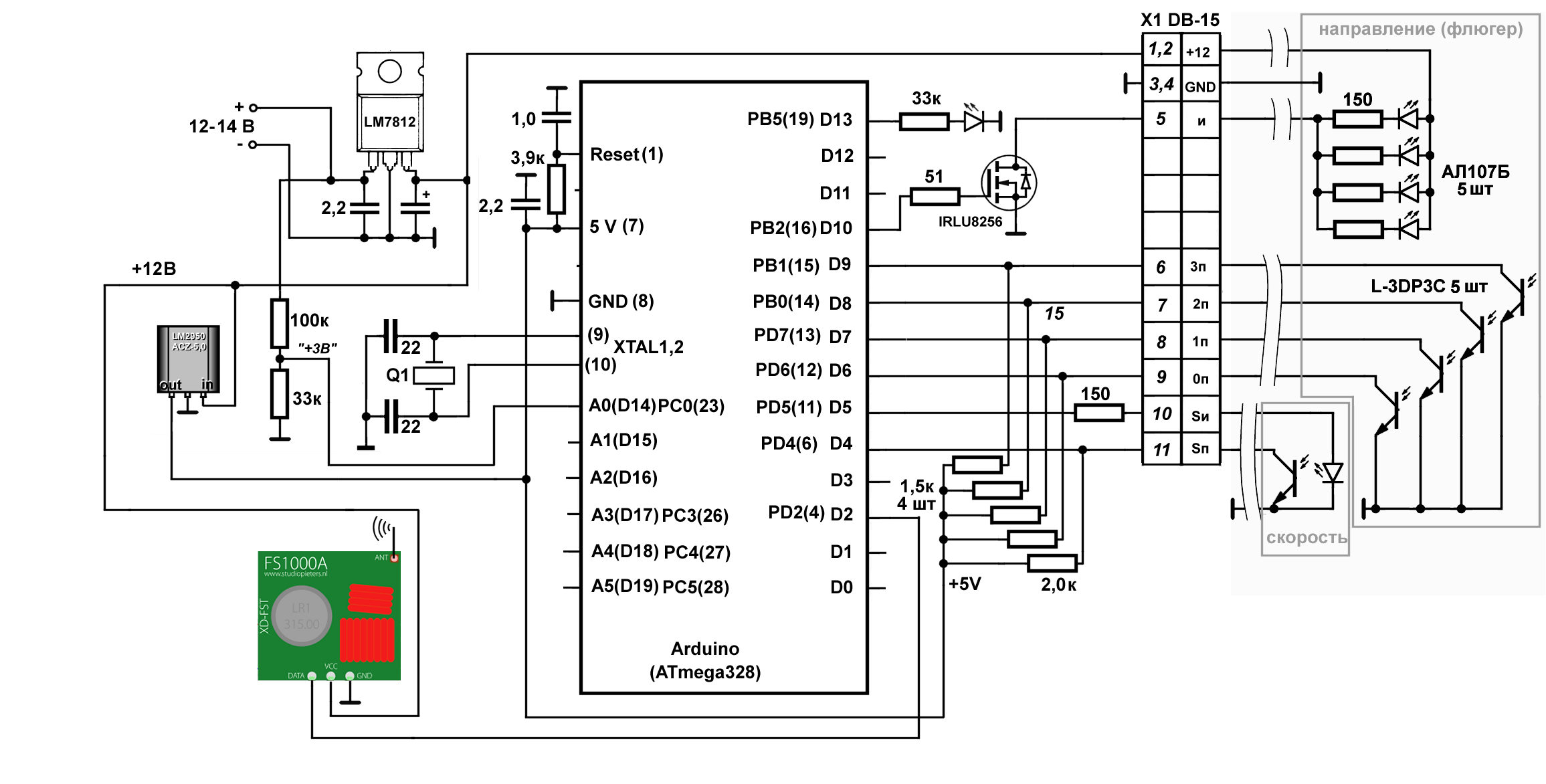
The schematic diagram of the wind sensor processing unit is as follows:
About where the power is taken 12-14 volts, see below. In addition to the components indicated in the diagram, the remote unit contains a temperature-humidity sensor, which is not shown in the diagram. A voltage divider connected to pin A0 of the controller is designed to control the voltage of the power supply for the purpose of timely replacement. The LED connected to the traditional pin 13 (pin 19 of the DIP housing) is superbright, for its normal, non-glare glow, there is enough current in the milliampere fraction, which is ensured by the unusually high 33 kΩ resistor rating.
The scheme uses a “bare” Atmega328 controller in a DIP package, programmed via Uno and mounted on the panel. Such controllers with an Arduino downloader already recorded are sold, for example, in Chip-Dipe (or the downloader can be recorded independently ). Such a controller is convenient to program in a familiar environment, but, devoid of components on the board, it is, firstly, more economical, and secondly, it takes up less space. A full-fledged energy-saving mode could be obtained by getting rid of the bootloader too (and generally writing all the code in assembler :), but here it is not very relevant, and programming is unnecessarily complicated.
In the diagram, gray rectangles are circled with components related separately to the speed and direction channels. Consider the operation of the circuit as a whole.
The operation of the controller as a whole is controlled by the WDT watchdog timer enabled in the interrupt call mode. WDT takes the controller out of sleep at specified intervals. In case the timer is re-started in the called interrupt, the reset from scratch does not occur, all global variables remain at their values. This allows you to accumulate data from awakening to awakening and at some point to process them - for example, average.
At the beginning of the program, the following declarations of libraries and global variables are made (in order not to clutter the text of the already extensive examples, everything related to the temperature-humidity sensor is released here):
#include <VirtualWire.h> #include <avr/wdt.h> #include <avr/sleep.h> . . . . . #define ledPin 13 // (PB5 19 ATmega) #define IR_Pin 10 // IRLU (PB2 16 Atmega) #define in_3p 9 // 3 #define in_2p 8 // 2 #define in_1p 7 // 1 #define in_0p 6 // 0 #define IR_PINF 5 //(PD5,11) - #define IN_PINF 4 //(PD4,6) volatile unsigned long ttime = 0; // float ff[4]; // char msg[25]; // byte count=0;// int batt[4]; // byte wDir[4]; // byte wind_Gray=0; //
To initiate sleep and WDT (wake up every 4 seconds), use the following procedures:
// void system_sleep() { ADCSRA &= ~(1 << ADEN); //. cbi(ADCSRA,ADEN); set_sleep_mode(SLEEP_MODE_PWR_DOWN); // sleep_mode(); // sleep_disable(); // watchdog ADCSRA |= (1 << ADEN); /. sbi(ADCSRA,ADEN); } //**************************************************************** // ii: 0=16ms, 1=32ms,2=64ms,3=128ms,4=250ms,5=500ms // 6=1 sec,7=2 sec, 8=4 sec, 9= 8sec void setup_watchdog(int ii) { byte bb; if (ii > 9 ) ii=9; bb=ii & 7; if (ii > 7) bb|= (1<<5); // bb - bb|= (1<<WDCE); MCUSR &= ~(1<<WDRF); // WDTCSR |= (1<<WDCE) | (1<<WDE); // WDTCSR = bb; WDTCSR |= (1<<WDIE); // WDT } //**************************************************************** // ISR(WDT_vect) { wdt_reset(); }
The speed sensor outputs the frequency of interruption of the optical channel, the order of magnitude - units-tens of hertz. To measure such a value more economically and faster through the period (this was the subject of the publication of the author “ Evaluation of methods for measuring low frequencies on the Arduino ”). Here, the method is selected through the modified pulseInLong () function, which does not bind the measurement to specific controller outputs (the text of the periodInLong () function can be found in the specified publication).
The setup () function declares the directions of the outputs, initializes the 433 MHz transmitter library and the watchdog timer (the IN_PINF line is, in principle, superfluous, and inserted for the memory):
void setup() { pinMode(IR_PINF, OUTPUT); // pinMode(IN_PINF, INPUT); // pinMode(13, OUTPUT); // vw_setup(1200); // VirtualWire vw_set_tx_pin(2); //D2, PD2(4) VirtualWire // Serial.begin(9600); // Serial- setup_watchdog(8); //WDT 4 c wdt_reset(); }
Finally, in the main program loop, we first, every time we wake up (every 4 seconds), read the voltage and calculate the frequency of the wind speed sensor:
void loop() { wdt_reset(); // digitalWrite(ledPin, HIGH); // batt[count]=analogRead(0); // /*=== ==== */ digitalWrite(IR_PINF, HIGH); // - float f=0; // ttime=periodInLong(IN_PINF, LOW, 250000); // 0,25 // Serial.println(ttime); // if (ttime!=0) {// f = 1000000/float(ttime);} // digitalWrite(IR_PINF, LOW); // - ff[count]=f; // . . . . .
The burning time of the IR LED (consuming, recall, 20 mA) here, as you can see, will be maximum if there is no rotation of the sensor disk and, under this condition, is about 0.25 seconds. The minimum measured frequency, therefore, will be 4 Hz (a quarter of a disk revolution per second with 16 holes). As it turned out when calibrating the sensor (see below), this corresponds to approximately 0.2 m / s wind speed. We emphasize that this is the minimum measured value of the wind speed, but not the resolution and not the starting point (which will be much higher). If there is a frequency (that is, when the sensor rotates), the measurement time (and, accordingly, the LED burning time, that is, the current consumption) will decrease proportionally, and the resolution will increase.
This is followed by the procedures that are performed every fourth awakening (that is, every 16 seconds). The value of the frequency of the speed sensor of the accumulated four values, we pass not the average, but the maximum - as experience has shown, this is a more informative value. Each of the values, regardless of its type, for convenience and uniformity, we turn into a positive integer with a size of 4 decimal places before transmission. The count variable keeps track of the number of awakenings:
// 16 // 4- : if (count==3){ f=0; // for (byte i=0; i<4; i++) if (f<ff[i]) f=ff[i]; // int fi=(int(f*10)+1000); // 4 . int volt=0; // for (byte i=0; i<4; i++) volt=volt+batt[i]; volt=volt/4+100; // 100 = 3 . volt=volt*10; // 4 . . . . . .
Next is the definition of the Gray direction code. Here, to reduce consumption, instead of the permanently on IR LEDs, all four channels are simultaneously fed through the key field-effect transistor using the tone () function and a frequency of 5 kHz is applied. Detection of the presence of frequency on each of the digits (in_0p - in_3p pins) is made by the method similar to the anti-rattle when reading the pressed button. First, we wait in the loop if there is a high level at the output, and then check it after 100 μs. 100 μs is a half-frequency of 5 kHz, that is, if there is a frequency at least the second time, we will again get to a high level (we repeat four times just in case) and this means that it is exactly there. We repeat this procedure for each of the four bits of the code:
/* ===== Wind Gray ==== */ //: tone(IR_Pin,5000);// 5 boolean yes = false; byte i=0; while(!yes){ // 3 i++; boolean state1 = (digitalRead(in_3p)&HIGH); delayMicroseconds(100); // 100 yes=(state1 & !digitalRead(in_3p)); if (i>4) break; // } if (yes) wDir[3]=1; else wDir[3]=0; yes = false; i=0; while(!yes){ // 2 i++; boolean state1 = (digitalRead(in_2p)&HIGH); delayMicroseconds(100); // 100 yes=(state1 & !digitalRead(in_2p)); if (i>4) break; // } if (yes) wDir[2]=1; else wDir[2]=0; yes = false; i=0; while(!yes){ // 1 i++; boolean state1 = (digitalRead(in_1p)&HIGH); delayMicroseconds(100); // 100 yes=(state1 & !digitalRead(in_1p)); if (i>4) break; // } if (yes) wDir[1]=1; else wDir[1]=0; yes = false; i=0; while(!yes){ // 0 i++; boolean state1 = (digitalRead(in_0p)&HIGH); delayMicroseconds(100); // 100 yes=(state1 & !digitalRead(in_0p)); if (i>4) break; // } if (yes) wDir[0]=1; else wDir[0]=0; noTone(IR_Pin); // // : wind_Gray=wDir[0]+wDir[1]*2+wDir[2]*4+wDir[3]*8; // . int wind_G=wind_Gray*10+1000; // 4- . . . . . .
The maximum duration of one procedure will be in the absence of frequency at the receiver and is equal to 4 × 100 = 400 microseconds. The maximum burning time of 4 direction LEDs will be when no receiver is illuminated, that is, 4 × 400 = 1.6 milliseconds. The algorithm, by the way, will work in the same way if, instead of the frequency, the period of which is a multiple of 100 µs, just submit a constant high level to the LEDs. In the presence of a meander instead of a constant level, we simply save food by half. We can save even more if we get each IR LED through a separate line (respectively, through a separate controller output with its own key transistor), but this also complicates the circuit, wiring and control, and the current is 130 mA for 2 ms every 16 seconds - this is, you see, a little.
Finally, wireless data transmission . To transfer data from the sensor installation site to the weather station display, the simplest, cheapest and most reliable method was chosen: a transmitter / receiver pair at a frequency of 433 MHz . I agree that the method is not the most convenient (due to the fact that the devices are designed to transfer bit sequences, rather than whole bytes, you have to refine your data conversion between the necessary formats), and I am sure that many will want to argue with me in terms of its reliability. The answer to the last objection is simple: “you just do not know how to cook them!”.
The secret is that it usually remains beyond the frame of various descriptions of data exchange over the 433 MHz channel: since these devices are purely analog, the receiver power must be very well cleaned of any extraneous pulsations. In no case should not power the receiver from the internal 5-volt Arduino stabilizer! Installation for the receiver of a separate low-power stabilizer (LM2931, LM2950 or similar) directly in the vicinity of its findings, with the correct filtering circuits at the input and output, dramatically increases the range and reliability of transmission.
In this case, the transmitter worked directly from the battery voltage of 12 V, the receiver and the transmitter were equipped with standard homemade antennas in the form of a 17 cm long wire. (Let me remind you that the antenna wire is only single-core, and the antennas should be placed in space parallel to each other.) A packet of information of 24 bytes in length (taking into account humidity and temperature) without any problems was confidently transmitted at a speed of 1200 bps diagonally across the 15 hectare garden plot (about 40-50 meters), and then after three logs walls inside the room (in which, for example, the cellular signal is received with great difficulty and not everywhere). Conditions practically unattainable for any standard 2.4 GHz method (such as Bluetooth, Zig-Bee, and even amateur Wi-Fi), while the transmitter consumption here is a measly 8 mA and only at the moment of transmission, the rest of the time the transmitter consumes penny. The transmitter is structurally placed inside the remote unit, the antenna sticks out laterally horizontally.
We combine all the data into one packet (in a real station, temperature and humidity will be added to it), consisting of uniform 4-byte parts and preceded by the “DAT” signature, send it to the transmitter and complete all the cycles:
/*=====Transmitter=====*/ String strMsg="DAT"; // - strMsg+=volt; // 4 strMsg+=wind_G; // wind 4 strMsg+=fi; // 4 strMsg.toCharArray(msg,16); // // Serial.println(msg); // vw_send((uint8_t *)msg, strlen(msg)); // vw_wait_tx(); // - ! delay(50); //+ count=0; // }//end count==3 else count++; digitalWrite(ledPin, LOW); // system_sleep(); // — } //end loop
The packet size can be reduced if the requirement to represent each of the values of various types in the form of a uniform 4-byte code is refused (for example, one byte is enough for the Gray code, of course). But for the sake of universalization, I left everything as it is.
Power and design features of the remote unit . The consumption of the remote unit is calculated as follows:
- 20 mA (emitter) + ~ 20 mA (controller with auxiliary circuits) for about 0.25 every four seconds - on average 40/16 = 2.5 mA;
- 130 mA (emitters) + ~ 20 mA (controller with auxiliary circuits) for about 2 ms every 16 seconds - an average of 150/16/50 ≈ 0.2 mA;
Drawing on this calculation, the consumption of the controller when removing data from the temperature-humidity sensor and when the transmitter is working, we can safely bring the average consumption to 4 mA (at a peak of about 150 mA, notice!). The batteries (which, by the way, will require as many as 8 pieces to provide the transmitter with the maximum voltage!) Will have to be changed too often, because the idea arose of supplying the remote unit with 12-volt batteries for the screwdriver - I just got two of them superfluous. Their capacity is even less than the corresponding number of AA batteries - only 1.3 A • hours, but no one bothers to change them at any time, keeping the second charged at the ready. With the indicated consumption of 4 mA, the capacity of 1300 mA • hours is enough for about two weeks, which is not too troublesome.
Note that the voltage of a freshly charged battery can be up to 14 volts. In this case, an input stabilizer of 12 volts is installed - in order to prevent overvoltages of the transmitter power supply and not to overload the main five-volt stabilizer.
The remote unit in a suitable plastic case is placed under the roof, to it on the connectors summed up the power cable from the battery and the connection to the wind sensors. The main difficulty is that the circuit turned out to be extremely sensitive to the humidity of the air: in rainy weather, after a couple of hours, the transmitter begins to fail, the frequency measurements show a complete mess, and the battery voltage measurements show the “weather on Mars”.
Therefore, after debugging the algorithms and checking all the connections, the housing must be carefully sealed. All connectors at the entrance to the housing are coated with a sealant, the same applies to all screw heads protruding to the outside, the antenna output and the power cable. The joints of the case are plastered with plasticine (taking into account the fact that they will have to be separated), and additionally are glued on top with strips of sanitary tape. It is not bad to additionally strengthen the used connectors inside with epoxy: for example, the DB-15 module shown on the diagram of the external module is not sealed by itself, and moist air will slowly seep between the metal frame and the plastic base.
But all these measures by themselves will only give a short-term effect - even if there is no cold humid air suction, the dry air from the room easily turns into wet when the temperature outside the case falls (think of a phenomenon called “dew point”).
To avoid this, it is necessary to leave the cartridge or bag with a desiccant - silica gel inside the case (bags with it are sometimes put in boxes with shoes or in some packages with electronic devices). If the silica gel is of unknown origin and has been stored for a long time, it must be calcined in an electric oven at 140-150 degrees for several hours before use. If the case is sealed properly, then the desiccant will have to be changed no more than at the beginning of each summer season.
The main module
In the main module, all values are accepted, decoded, if necessary, converted in accordance with the calibration equations and displayed on the display.
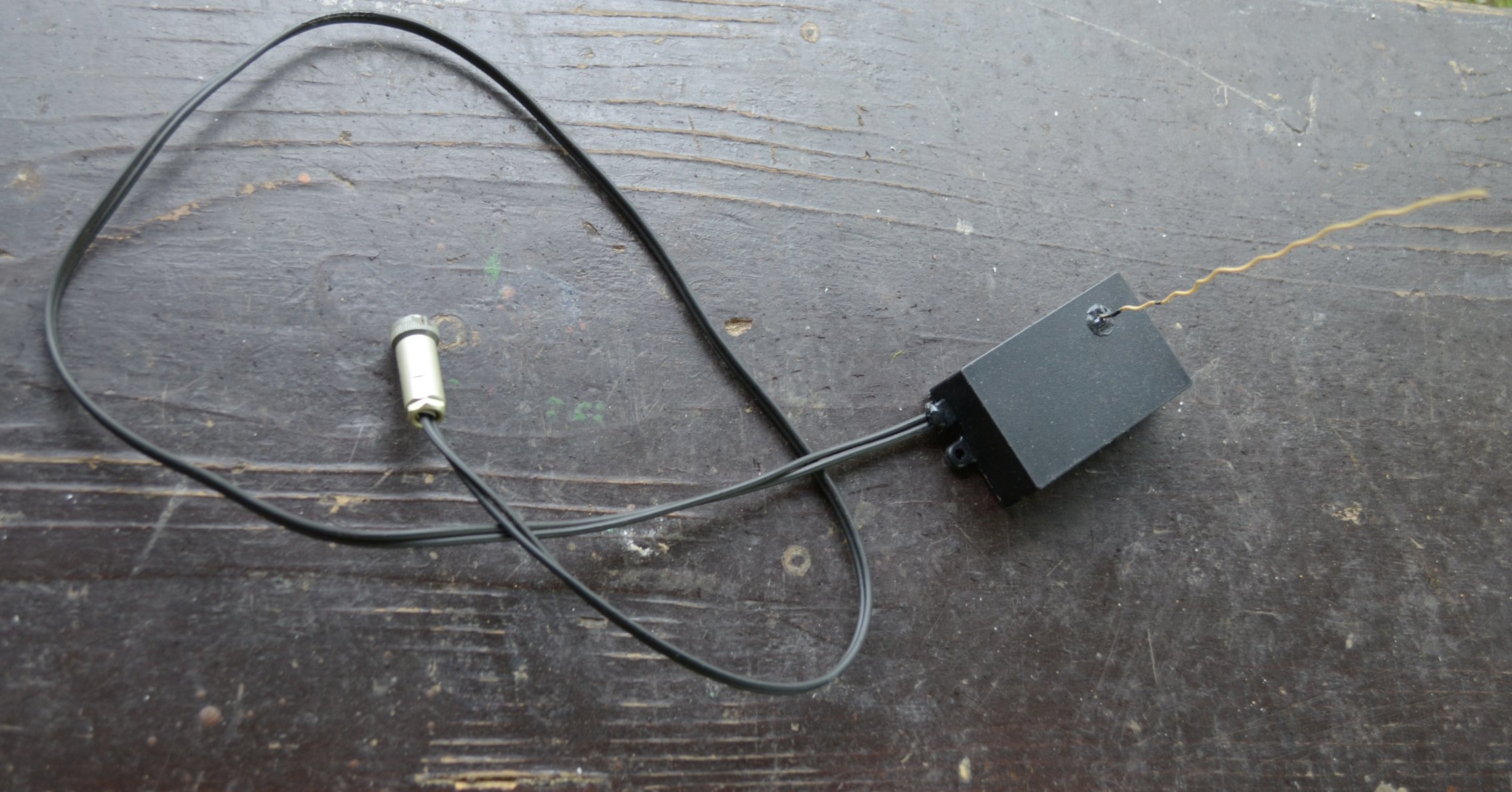
The receiver is located outside the main module of the station and placed in a small box with ears for mounting. The antenna is brought out through the hole in the cover, all the holes in the body are sealed with wet rubber. The contacts of the receiver are brought to a very reliable domestic PC-4 type connector, from the receiver side it is connected through a piece of shielded dual AV cable:
A signal is picked up along one of the cable cores, the other is supplied with raw 9 volts from the module power adapter. The stabilizer type LM-2950-5.0 with filtering capacitors installed in a box with the receiver on a separate scarf.
Experiments were carried out to increase the length of the cable (just in case - suddenly it wouldn't work through the wall?), In which it turned out that nothing changes within the limits of length up to 6 meters.
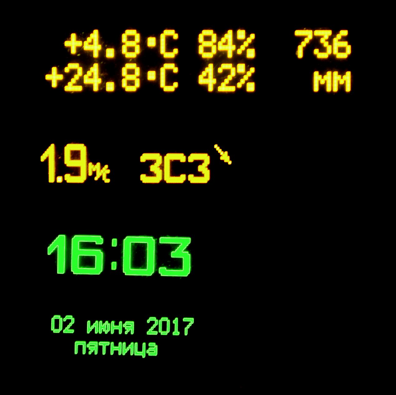
There are only four OLED displays: two yellow serve weather data, two green clocks and a calendar. Their placement is shown in the photo:
Please note that in each group one of the displays is text, the second is graphic, with artificially created fonts in the form of glyph pictures. Here we will not dwell on the issue of displaying information on displays in order not to inflate the already extensive text of the article and examples: due to the presence of glyph pictures that have to be output individually (often simply by enumerating options by the case statement), output programs can be very cumbersome. For information on how to handle such displays, see the author’s publication Graphic and Text Mode of Winstar Displays , including an example of a display for displaying wind data.
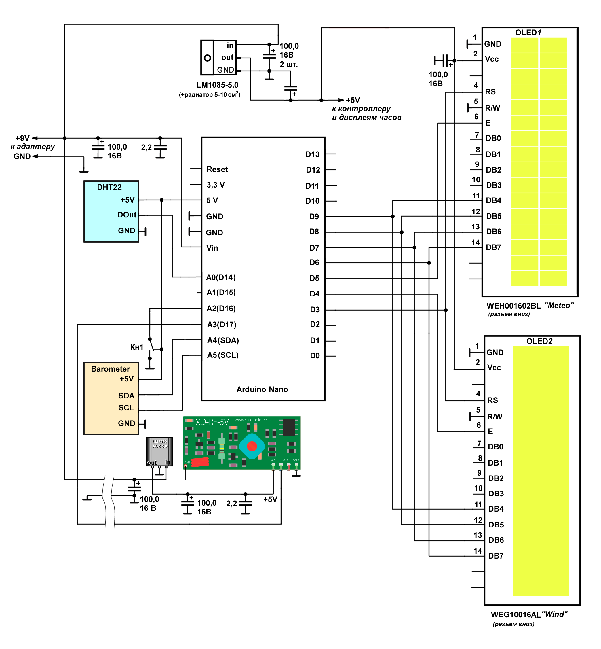
Schematic diagram. For convenience, the clocks and their displays are serviced by a separate Arduino Mini controller and we will not analyze them anymore. The scheme of connecting components to Arduino Nano, which controls the reception and output of weather data, is as follows:
Here, unlike the remote module, the connection of weather sensors - a barometer and an internal temperature-humidity sensor is shown. Attention should be paid to the power wiring - the displays are powered by a separate 5 V stabilizer type LM1085. It is natural to power the clock displays from it, but in this case the clock controller should also be powered from the same voltage, moreover, via the 5 V output, not Vin (for the Mini Pro, the latter is called RAW). If the clock controller is powered the same way as the Nano - 9 volts via the RAW pin, then its internal stabilizer will conflict with the external 5 volts and in this fight, naturally, the strongest will win, that is LM1085, and the Mini will remain completely without power. Also, in order to avoid all sorts of trouble, before programming Nano and especially Mini (that is, before connecting the USB cable), the external adapter should be disconnected.
On the LM1085 stabilizer, when all four displays are connected, power will be released about a watt, so it should be installed on a small radiator around 5-10 cm2 from an aluminum or copper corner.
Reception and data processing. Here I am reproducing and commenting only fragments of the program relating to wind data, on the other sensors, a few words further.
To receive messages on the 433 MHz channel, we apply the standard method described in many sources. We connect the library and declare variables:
#include <VirtualWire.h> . . . . . int volt; // float batt; // — byte wDir; // uint16_t t_time = 0; // char str[5]; // uint8_t buf[VW_MAX_MESSAGE_LEN]; // uint8_t buflen = VW_MAX_MESSAGE_LEN; // max . . . . .
One feature is connected with the size of the buffer buflen: it is not enough to declare its value (VW_MAX_MESSAGE_LEN) once at the beginning of the program. Since this variable appears in the receive function (see below) by reference, the default message size has to be updated each cycle. Otherwise, due to the reception of corrupted messages, the value of buflen will be shortened each time until you start receiving nonsense instead of data. In the examples, both of these variables are usually declared locally in the loop (), because the buffer size is updated automatically, and here we will simply repeat the assignment of the desired value at the beginning of each loop.
In the setup procedure, we make the following settings:
void setup() { delay (500); // pinMode(16,INPUT_PULLUP); // vw_setup(1200); // VirtualWire vw_set_rx_pin(17); //A3 VirtualWire . . . . .
, - , t_time, . (, 48 — ), , - :
void loop() { vw_rx_start(); // buflen = VW_MAX_MESSAGE_LEN; // if ((int(millis()) - t_time) > 48000) // t_time 48 { < > }//end if (vw_have_message()) { // if (vw_get_message(buf, &buflen)) // { vw_rx_stop(); // t_time = millis(); // t_time for (byte i=0;i<3;i++) // str[i]= buf[i]; str[3]='\0'; if((str[0]=='D')&&(str[1]=='A')&&(str[2]=='T')) { // // : for (byte i=3;i<7;i++) // str[i-11]= buf[i]; // volt=atoi(str); // volt=(volt/10)-100; // 4- batt=float(volt)/55.5; // // for (byte i=7;i<11;i++) // str[i-15]= buf[i]; // int w_Dir=atoi(str); // w_Dir=(w_Dir-1000)/10; // wDir=lowByte(w_Dir); // - < case> . . . . .
55.5 — , .
, : , . , . , - — , («», «», «», «», «» ..), . , .
, , :
. . . . . for (byte i=19;i<23;i++) // str[i-19]= buf[i]; // int wFrq=atoi(str); // wFrq = (wFrq-1000)/10; // 4- wFrq=10+0.5*wFrq;// < > }//end if str=DAT }//end vw_get_message } //end vw_have_message(); . . . . .
10+0.5*wFrq — . 10 / ( 1.0 ) , 0,5 — ( /). 10 /, , 1 /, . . — , - V F: V = V + K×F , , V ( ).
, , . , — . 1 — , ( ) - :
. . . . . if (digitalRead(16)==LOW){ // < , -> }// delay(500); }// loop
, , , , . , , , 10 , , .
. SHT-75 — , « » ( ).
.
SHT-75 -: , . ATmega328 , , . , 20-130 ( ) SHT-75 , , .
SHT-75 , , 433 . 4- .
DHT-22 — , , (, , DHT-11, , ). DHT-22 ( SHT-75 !), SHT-75. .
, DHT-22 — . , . , , , ( ) , RST Oregon , ( ) - .
, — (MEMS) BMP180 . LPS331AP : , I2C-. , , — 10-12 1 .. Art. ( ) , .
— , . , .
UPD 30.06.17. . :
controller
Battery
+ 2,5 . .
, . 3 ( ), :
«3 24 6 = 12
3 24 3 = 24 »
No comments.
In my case, the resulting power of a solar power plant is dozens of times higher than necessary in the worst weather conditions. Therefore, in the sensor controller, you can not particularly care about energy saving, and apply any necessary frequency of reading and averaging values.
UPD from 09/13/18. For almost two seasons of operation, the strengths and weaknesses of the station were revealed. The weak ones are first of all the fact that the cycle of updating the readings in 16 seconds (out of four series of measurements), as it was originally, is too long. Installing a solar battery with a buffer battery made it possible not to think about energy saving and play around with the duration of the cycle. As a result, the cycle was set to 8 seconds (four measurements in two seconds).
(, , , ). ( , , ). , . , - , , , . , : , , .
The main change in calculation algorithms also applies to wind sensors, and I found it useful to put it in a separate article .
All Articles