プログラマーが車を買った方法

最近、中古の検索に困惑しました 車を販売するだけでなく、通常のように、いくつかの競合他社がこの役割を主張しています。



ご存知のように、ロシア連邦で車を購入するために、いくつかの大きな評判の良いサイト（auto.ru、drom.ru、avito.ru）がありますが、検索を優先しました。 上記のサイトの何百台、および一部のモデルと数千台の車が私の要件を満たしていました。 いくつかのリソースで検索するのは不便であるという事実に加えて、車を「ライブ」で見る前に、各リソースが提供するアプリオリ情報に有利な（市場よりも価格が低い）オファーを選択したいと思います。 もちろん、高次元の代数方程式（非線形の可能性もある）のいくつかの過剰決定システムを手動で解決したかったのですが、私は自分自身を圧倒し、このプロセスを自動化することにしました。

データ収集

上記のすべてのリソースからデータを収集しましたが、次のパラメーターに興味がありました。

• 価格
• 製造年（年）
• 走行距離
• エンジン量（engine.capacity）
• エンジン出力（engine.power）
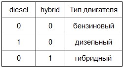
• エンジンの種類（ディーゼルとハイブリッドの場合、それぞれ値0または1をとる2つのインジケーター、相互に排他的なディーゼルとハイブリッドの変数）。 デフォルトのエンジンタイプはガソリンです（ 多重共線性を避けるために3番目の変数に移動されません）。
  
  
  
  このように：
  
  
  
  
  
  
  
  さらに、インジケータ変数の同様のロジックがデフォルトで暗示されています。
• ギアボックスのタイプ（インジケータ変数mt（手動送信）。手動送信の場合はブール値を取ります）。 デフォルトのギアボックスタイプは自動です。
  
  
  
  オートマチックトランスミッションは、古典的な油圧機械だけでなく、ロボット機構とバリエーターにも起因していることに注意してください。
• ドライブタイプ（ブール値を受け入れる2つのインジケータ変数front.driveおよびrear.drive）。 デフォルトのドライブタイプはフルです。
• ボディタイプ（セダン、ハッチバック、ワゴン、クーペ、カブリオレ、ミニバン、ピックアップ、ブール値を取る7つのインジケーター変数）。 デフォルトのボディタイプはSUV /クロスオーバーです

Rを使用してこれらの値を正しく処理できるように、怠zyな売り手が入力していないデータをNA（使用不可）とマークしました。

データの可視化

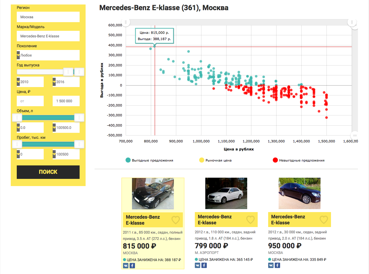
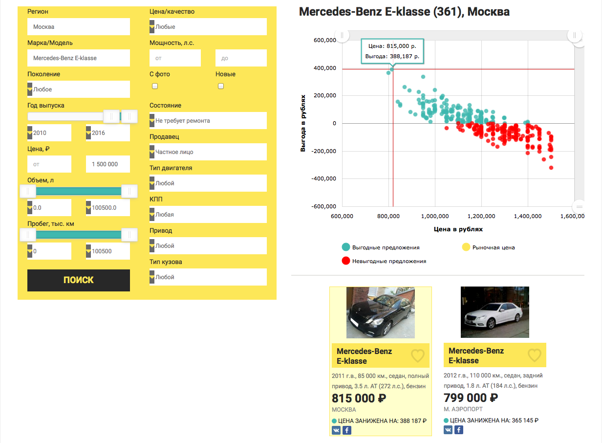
ドライ理論に進まないために、具体的な例を見てみましょう。モスクワで最大150万ルーブルの、2010年リリースよりも前の収益性の高いメルセデスベンツEクラスを探します。 データの操作を開始するには、まず、欠損値（NA）に中央値を入力します。幸いなことに、Rには中央値（）関数があります。

dat <- read.csv("dataset.txt") #    R

dat$mileage[is.na(dat$mileage)] <- median(na.omit(dat$mileage)) #   

      
      

        
        
        
      

    
        
        
        
      
      

        
        
        
      

    
    

, .



( ).







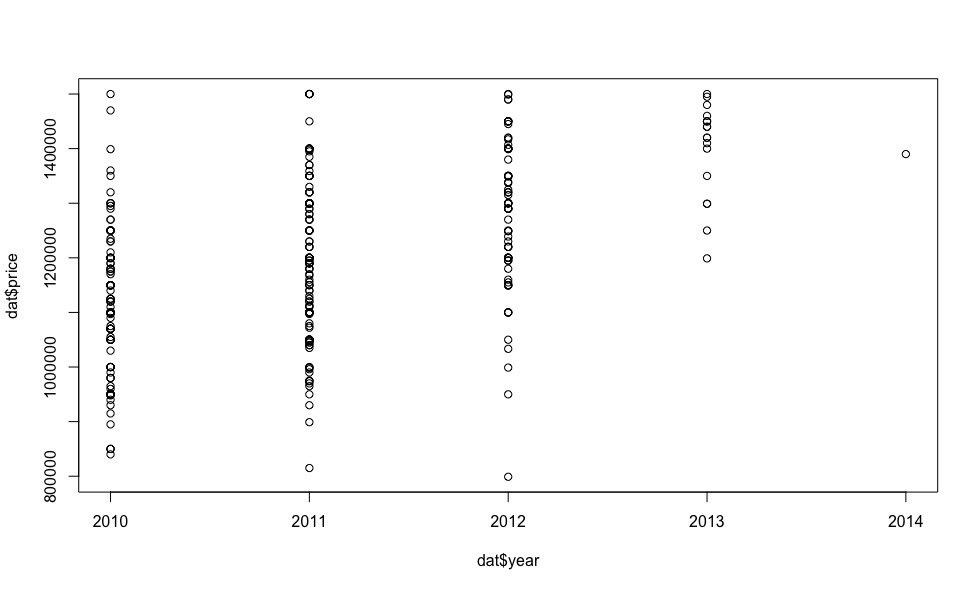
2013 2014!







, , .











— , , .



, , , “”, , .



, , .

, , , , .



, -:

1. , ..:
   
   
   • .
     
     
     
     
     (. ), .
     
     
     
     
     
   • .
     
     
     
     
     , :
     
     
     
     

     dat_cor <- as.matrix(cor(dat)) #    
     
     dat_cor[is.na(dat_cor)] <- 0 #     0 (..          )
     
     library(corrplot) #   corrplot,   
     
     palette <-colorRampPalette(c("#7F0000","red","#FF7F00","yellow","#7FFF7F", "cyan", "#007FFF", "blue","#00007F"))
     
     corrplot(dat_cor, method="color", col=palette(20), cl.length=21,order = "AOE", addCoef.col="green") #     
     
           
           
     
             
             
             
           
     
         
             
             
             
           
           
     
             
             
             
           
     
         
         

     
     
     
     
     
     
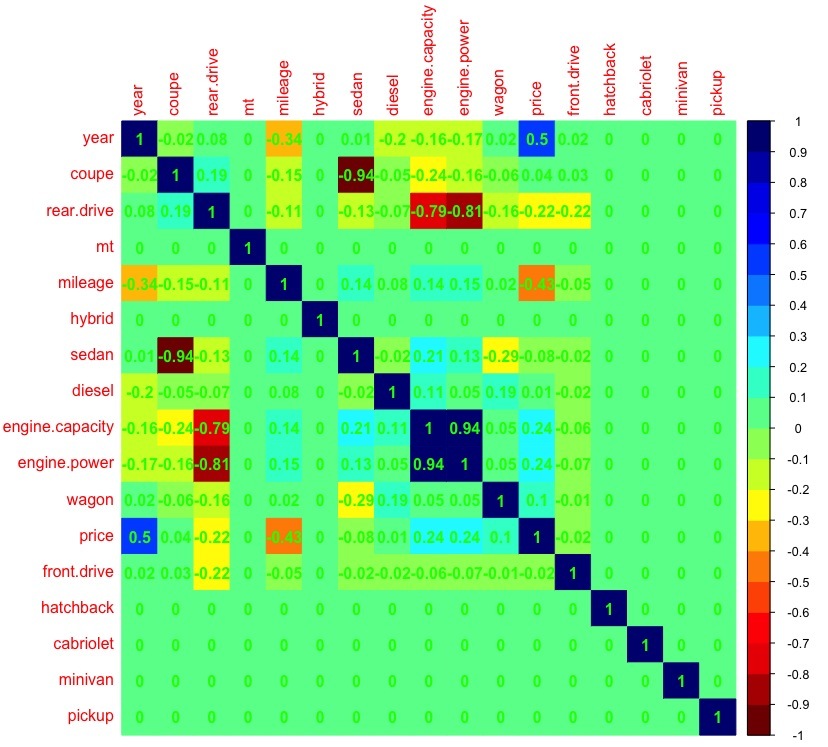
     (>0.7) , engine.capacity, .. ( , , — ).
     
     
     
     
     
   • .
     
     
     
     
     — (. ), . , , — , , , .
     
     
     
     . , , dffits, (covratio), , i- , . , dfbetas, i- .
     
     
     
     (covratio) — . i- .
     
     
     
     , , , dffits.
     
     
     
     — , .. , .
     
     , dffits covratio.
     
     
     
     

     model <- lm(price ~ year + mileage  + diesel + hybrid + mt + front.drive + rear.drive + engine.power + sedan + hatchback + wagon + coupe + cabriolet + minivan + pickup, data = dat) #  
     
     model.dffits <- dffits(model) #   dffits
     
           
           
     
             
             
             
           
     
         
             
             
             
           
           
     
             
             
             
           
     
         
         

     
     
     dffits 2*sqrt(k/n) = 0.42, (k — , n — ).
     
     
     
     

     model.dffits.we <- model.dffits[model.dffits < 0.42]
     
     model.covratio <- covratio(model)  #     
     
           
           
     
             
             
             
           
     
         
             
             
             
           
           
     
             
             
             
           
     
         
         

     
     
     covratio | model.covratio[i] -1 | > (3*k)/n.
     
     
     
     

     model.covratio.we <- model.covratio[abs(model.covratio -1) < 0.13]
     
     dat.we <- dat[intersect(c(rownames(as.matrix(model.dffits.we))), c(rownames(as.matrix(model.covratio.we)))),] #   
     
     model.we <- lm(price ~ year + mileage  + diesel + hybrid + mt + front.drive + rear.drive + engine.power + sedan + hatchback + wagon + coupe + cabriolet + minivan + pickup, data = dat.we) #       
     
           
           
     
             
             
             
           
     
         
             
             
             
           
           
     
             
             
             
           
     
         
         

     
     
     , , .
     
     
     
     
     
     
     
     
     
     
     
     
     
     
     
     , 18 , .
     
     
     
     
     
   
   
   
2. .
   
   
   
   
   .
   
   
   
   
   
3. , ()
   
   
   
   
   ( R resid()).
   
   
   
   

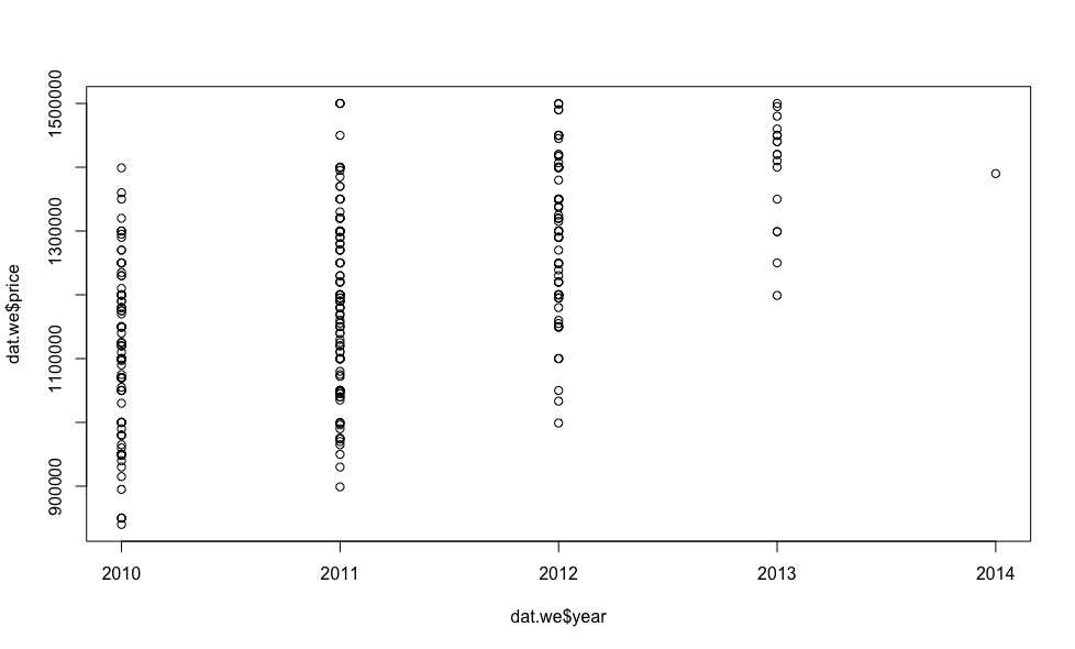
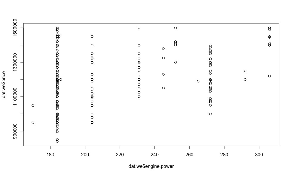
   plot(dat.we$year, resid(model.we))
   plot(dat.we$mileage, resid(model.we))
   plot(dat.we$engine.power, resid(model.we))
   
         
         
   
           
           
           
         
   
       
           
           
           
         
         
   
           
           
           
         
   
       
       

   
   
   
   
   
   
   
   
   
   
   
   
   
   
   - , .
   
   
   
   
   
4. .
   
   
   
   
   , , .
   
   
   
   

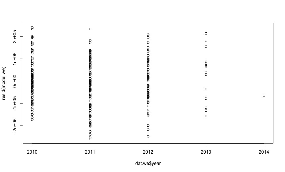
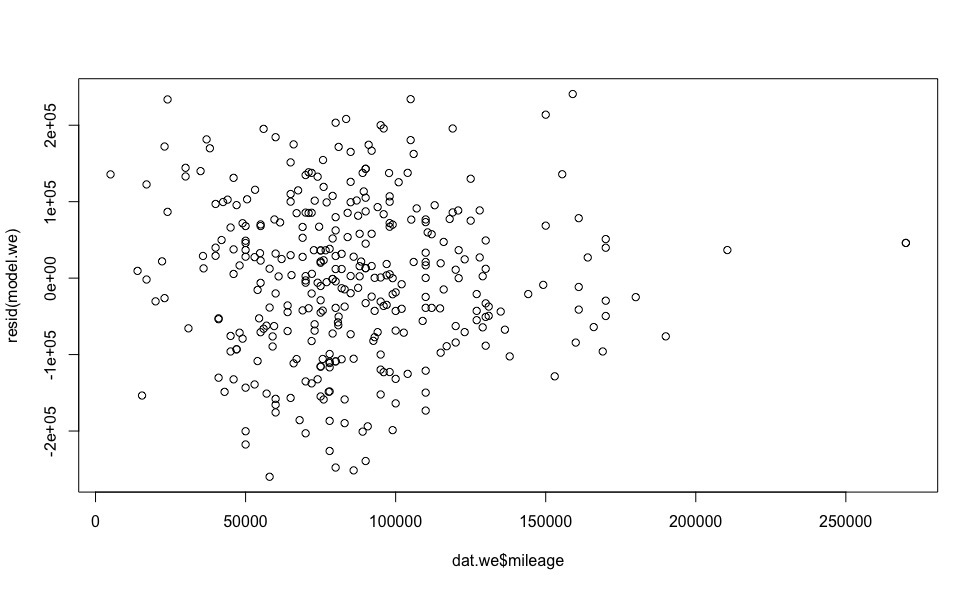
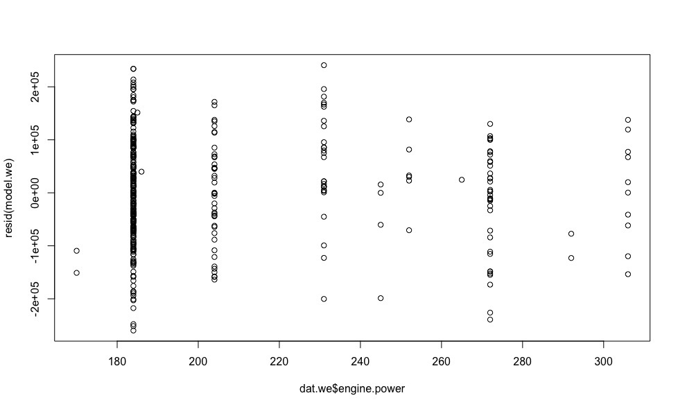
   qqnorm(resid(model.we)) 
   qqline(resid(model.we))
   
         
         
   
           
           
           
         
   
       
           
           
           
         
         
   
           
           
           
         
   
       
       

   
   
   
   
   

, , , . , , .

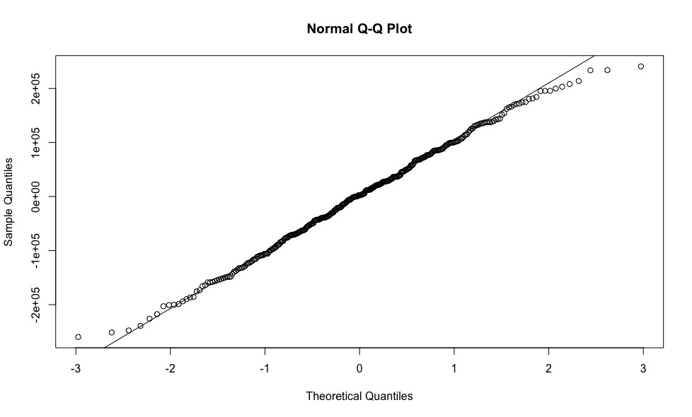
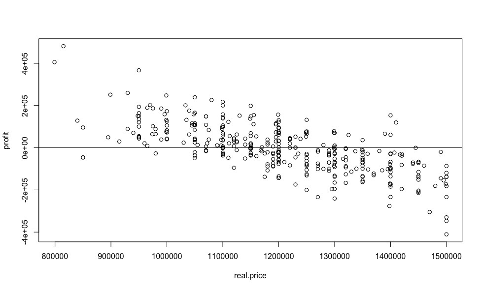
model.we <- lm(price ~ year + mileage  + diesel + hybrid + mt + front.drive + rear.drive + engine.power + sedan + hatchback + wagon + coupe + cabriolet + minivan + pickup, data = dat.we)

coef(model.we) #   
  (Intercept)  year  mileage  diesel  rear.drive  engine.power  sedan 
  -1.76e+08  8.79e+04  -1.4e+00  2.5e+04  4.14e+04  2.11e+03  -2.866407e+04        
    
predicted.price <- predict(model.we, dat) #     

real.price <- dat$price #       

profit <- predicted.price - real.price #         

      
      

        
        
        
      

    
        
        
        
      
      

        
        
        
      

    
    

, - , , , .

plot(real.price,profit)
abline(0,0)

      
      

        
        
        
      

    
        
        
        
      
      

        
        
        
      

    
    

?

sorted <- sort(predicted.price /real.price, decreasing = TRUE)
sorted[1:10]
      69       42      122      248      168       15      244      271      109      219 
1.590489 1.507614 1.386353 1.279716 1.279380 1.248001 1.227829 1.209341 1.209232 1.204062 

      
      

        
        
        
      

    
        
        
        
      
      

        
        
        
      

    
    

, 59% , , «», .. , . 4- ( 28%) , .



, , , , , (, , , , , , ), . , , , .

, , 3 :

1. ?
2. ?
3. ?

:

1. 80/20.
   
   
   
   

   set.seed(1) #     ( )
   
   split <- runif(dim(dat)[1]) > 0.2 #   
   
   train <- dat[split,] #   
   
   test <- dat[!split,] #  
   
   train.model <- lm(price ~ year + mileage  + diesel + hybrid + mt + front.drive + rear.drive + engine.power + sedan + hatchback + wagon + coupe + cabriolet + minivan + pickup, data = train) #       
   
   train.dffits <- dffits(train.model) #   dffits
   
   train.dffits.we <- train.dffits[train.dffits < 0.42] #     dffits 
   
   train.covratio <- covratio(train.model)  #     
   
   train.covratio.we <- model.covratio[abs(model.covratio -1) < 0.13] #     covratio 
   
   train.we <- dat[intersect(c(rownames(as.matrix(train.dffits.we))), c(rownames(as.matrix(train.covratio.we)))),] #     
   
   train.model.we <- lm(price ~ year + mileage  + diesel + hybrid + mt + front.drive + rear.drive + engine.power + sedan + hatchback + wagon + coupe + cabriolet + minivan + pickup, data = train.we) #         
   
   predictions <- predict(train.model.we, test) #     
   
   print(sqrt(sum((as.vector(predictions - test$price))^2)/length(predictions))) #     ( )
   [1] 121231.5
   
         
         
   
           
           
           
         
   
       
           
           
           
         
         
   
           
           
           
         
   
       
       

   
   
   — .
   
   
2. , , .
   
   
   
   2 ( ) .
   
   
   
   .
3. , -, .
   
   
   
   , — Mercedes-Benz E-klasse 2010 , 1.5 . .
   
   
   
   
   
   
   
   
   
   
   
   
   
   

1. csv — dataset.txt