Rの静的および動的ネットワークの視覚化、パート5

最初の部分で ：

• ネットワークの可視化：なぜですか？ どうやって？
• 視覚化オプション
• ベストプラクティス-美学とパフォーマンス
• データ形式と準備
• 例で使用されているデータセットの説明
• igraphを始めよう

第二部 ：R.チャートの色とフォント



3番目の部分：グラフ、頂点、およびエッジのパラメーター。



4番目の部分：ネットワークの場所。



このパートでは、ネットワーク、頂点、エッジ、パスのプロパティを強調します。

ネットワークプロパティの強調

ネットワークグラフはまだ有用ではないことに注意してください。 頂点のタイプとサイズを決定できますが、調査中のエッジが非常に近いため、構造についてはほとんど言えません。 問題を解決する1つの方法は、最も重要な接続のみを残し、残りを破棄して、ネットワークを「間引く」ことができるかどうかを確認することです。

hist(links$weight) mean(links$weight) sd(links$weight)
      
      

        
        
        
      

    
        
        
        
      
      

        
        
        
      

    
     

キーエッジを強調表示するより複雑な方法がありますが、この例では、重みがネットワークの平均値を超えるもののみを残します。 igraphでは、 delete.edges(net, edges)



を使用してエッジを削除できます。

 cut.off <- mean(links$weight) net.sp <- delete.edges(net, E(net)[weight<cut.off]) l <- layout.fruchterman.reingold(net.sp, repulserad=vcount(net)^2.1) plot(net.sp, layout=l)
      
      

        
        
        
      

    
        
        
        
      
      

        
        
        
      

    
     

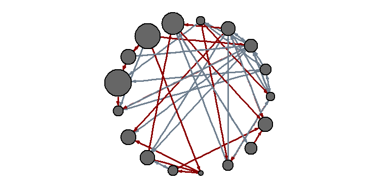
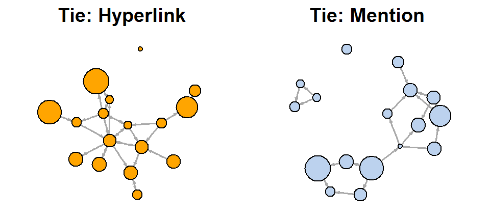
問題を解決する別のアプローチは、2種類のリンク（リンクと参照）を別々に導出することです。

 E(net)$width <- 1.5 plot(net, edge.color=c("dark red", "slategrey")[(E(net)$type=="hyperlink")+1], vertex.color="gray40", layout=layout.circle)
      
      

        
        
        
      

    
        
        
        
      
      

        
        
        
      

    
     

 net.m <- net - E(net)[E(net)$type=="hyperlink"] #     net.h <- net - E(net)[E(net)$type=="mention"] par(mfrow=c(1,2)) plot(net.h, vertex.color="orange", main="Tie: Hyperlink") # :  plot(net.m, vertex.color="lightsteelblue2", main="Tie: Mention") # : 
      
      

        
        
        
      

    
        
        
        
      
      

        
        
        
      

    
     

 l <- layout.fruchterman.reingold(net) plot(net.h, vertex.color="orange", layout=l, main="Tie: Hyperlink") plot(net.m, vertex.color="lightsteelblue2", layout=l, main="Tie: Mention")
      
      

        
        
        
      

    
        
        
        
      
      

        
        
        
      

    
     

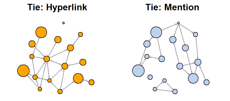
 dev.off()
      
      

        
        
        
      

    
        
        
        
      
      

        
        
        
      

    
     

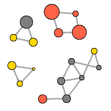
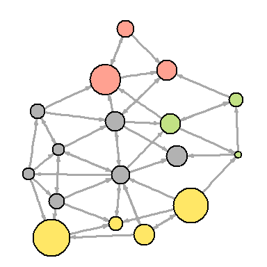
また、ネットワークマップに関連付けを表示することで、ネットワークマップをさらに便利にすることもできます。

 V(net)$community <- optimal.community(net)$membership colrs <- adjustcolor( c("gray50", "tomato", "gold", "yellowgreen"), alpha=.6) plot(net, vertex.color=colrs[V(net)$community])
      
      

        
        
        
      

    
        
        
        
      
      

        
        
        
      

    
     

いくつかの頂点またはエッジのアクセント

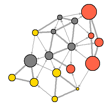
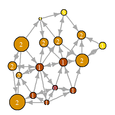
特定の頂点または頂点のグループに視覚化を集中する必要がある場合があります。 この例のメディアネットワークでは、中央サイト間の情報の分布を調べることができます。 たとえば、NYT（New York Times）からの距離を導き出しましょう。 shortest.paths



関数（名前が示すとおり）は、ネットワーク内のノード間の最短パスのマトリックスを返します。

 dist.from.NYT <- shortest.paths(net, algorithm="unweighted")[1,] oranges <- colorRampPalette(c("dark red", "gold")) col <- oranges(max(dist.from.NYT)+1)[dist.from.NYT+1] plot(net, vertex.color=col, vertex.label=dist.from.NYT, edge.arrow.size=.6, vertex.label.color="white")
      
      

        
        
        
      

    
        
        
        
      
      

        
        
        
      

    
     

または、WSJ（Wall Street Journal）のすべての最も近い隣人を表示できます。 neighbors



関数は、中央オブジェクトから1ステップですべての頂点を見つけることに注意してください。 ノードのすべてのエッジを検出する同様の関数は、 incident



と呼ばれます。

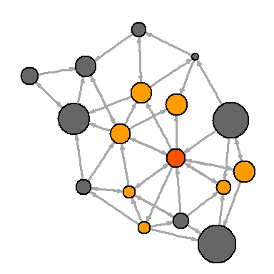
 col <- rep("grey40", vcount(net)) col[V(net)$media=="Wall Street Journal"] <- "#ff5100" neigh.nodes <- neighbors(net, V(net)[media=="Wall Street Journal"], mode="out") col[neigh.nodes] <- "#ff9d00" plot(net, vertex.color=col)
      
      

        
        
        
      

    
        
        
        
      
      

        
        
        
      

    
     

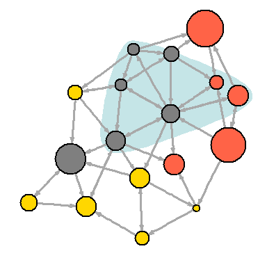
頂点のグループに注意を引くもう1つの方法は、頂点に「タグを付ける」ことです。

 plot(net, mark.groups=c(1,4,5,8), mark.col="#C5E5E7", mark.border=NA)
      
      

        
        
        
      

    
        
        
        
      
      

        
        
        
      

    
     

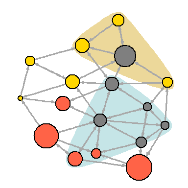
 #   : plot(net, mark.groups=list(c(1,4,5,8), c(15:17)), mark.col=c("#C5E5E7","#ECD89A"), mark.border=NA)
      
      

        
        
        
      

    
        
        
        
      
      

        
        
        
      

    
     

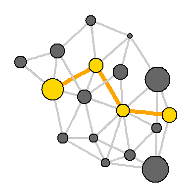
ネットワークパスを強調表示することもできます。

 news.path <- get.shortest.paths(net, V(net)[media=="MSNBC"], V(net)[media=="New York Post"], mode="all", output="both") #    : ecol <- rep("gray80", ecount(net)) ecol[unlist(news.path$epath)] <- "orange" #    : ew <- rep(2, ecount(net)) ew[unlist(news.path$epath)] <- 4 #    : vcol <- rep("gray40", vcount(net)) vcol[unlist(news.path$vpath)] <- "gold" plot(net, vertex.color=vcol, edge.color=ecol, edge.width=ew, edge.arrow.mode=0)