最初の写真は蓮を示しています。 この図は、Wolfram Mathematicaプログラムに組み込まれています。
コード
phi = 0; dphi = 2*Pi/7; theta[r_] := 0.4*r; theta1[r_] := 1*r; theta2[r_] := 0.7*r; Show[ ParametricPlot3D[{r*Cos[phi], r*Sin[phi], 0}, {r, 0, 0.8}, {phi, 0, 2 Pi}, PlotStyle -> Darker[Green], Mesh -> None], ParametricPlot3D[{r*Cos[phi], r*Sin[phi], 0.02}, {r, 0, 0.15}, {phi, 0, 2 Pi}, PlotStyle -> Yellow, Mesh -> None], ParametricPlot3D[ Join[ Table[ {r*Cos[theta[r]]*Cos[(i*dphi) + t*dphi/2*r*(1 - r)^1.5*5], r*Cos[theta[r]]*Sin[(i*dphi) + t*dphi/2*r*(1 - r)^1.5*5], r*Sin[theta[r]]}, {i, 0, 6}], Table[{r*Cos[theta1[r]]*Cos[(i*dphi) + t*dphi/2*r*(1 - r)^1.5*5], r*Cos[theta1[r]]*Sin[(i*dphi) + t*dphi/2*r*(1 - r)^1.5*5], r*Sin[theta1[r]]}, {i, 0, 6}], Table[{r*Cos[theta2[r]]* Cos[(dphi/2 + i*dphi) + t*dphi/2*r*(1 - r)^1.5*5], r*Cos[theta2[r]]* Sin[(dphi/2 + i*dphi) + t*dphi/2*r*(1 - r)^1.5*5], r*Sin[theta2[r]]}, {i, 0, 6}]], {r, 0, 1}, {t, -1, 1}, PlotStyle -> Directive[Specularity[RGBColor[1, 0.3, 0], 20], RGBColor[0.972, 0.658, 0.898], Lighting -> {{"Directional", Darker[White, 0.5], {2, 0, 2}}, {"Ambient", Darker[White]}}], Mesh -> None], PlotRange -> {{-0.85, 0.85}, {-0.85, 0.85}, {0, 0.8}}]
これらの公式は、球面座標系で想像しやすいです:半径ベクトルの長さ
 緯度
緯度  、経度
、経度  。 ここに入力したパラメーター
  。 その意味は、経度でポイントを取ることです
  そしてそこから退く
  経度の減少と増加の方向に。
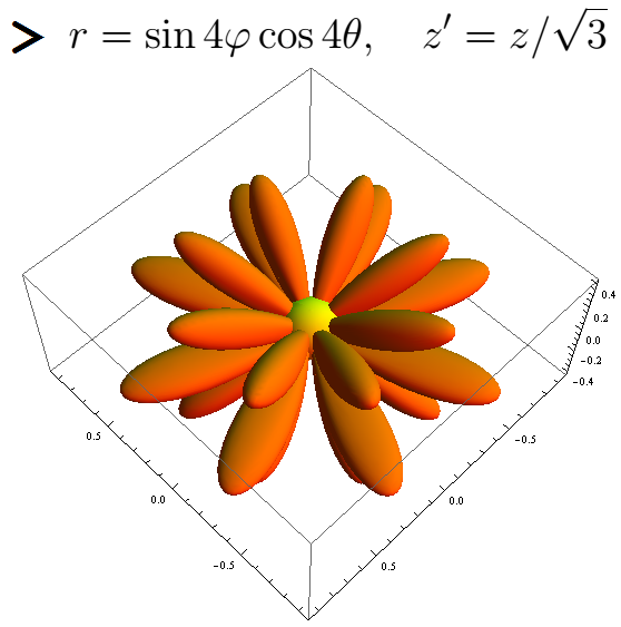
次の絵はきれいな花です。 式は球座標系で与えられ、 z軸に沿った圧縮変換も行われています。
コード
r[theta_, phi_] := If[(Pi/2 - Abs[theta] < Pi/8), 0.25*Sin[theta], Sin[4*phi]*Cos[4*theta]]; Show[ParametricPlot3D[ {r[theta, phi]*Cos[theta]*Cos[phi], r[theta, phi]*Cos[theta]*Sin[phi], r[theta, phi]*Sin[theta]/Sqrt[3]}, {theta, -Pi/2, Pi/2}, {phi, 0, 2*Pi}, Mesh -> None, PlotStyle -> Orange, PlotRange -> All, MaxRecursion -> 4], SphericalPlot3D[0.16, theta, phi, Mesh -> None, PlotStyle -> Yellow]]
ここに別の花があります。
コード
xx[t_] := 0; yy[t_] := -0.75 t*(1 - t); zz[t_] := -3 t; rr = 0.05; x1[t_] := 0; y1[t_] := -0.15 + 0.5 t; z1[t_] := -1.6 + 0.5 t; r[theta_, phi_] := If[(Pi/2 - Abs[theta] < Pi/8), 0.25*Sin[theta], Sin[4*phi]*Cos[4*theta]]; Show[ParametricPlot3D[ {r[theta, phi]*Cos[theta]*Cos[phi], r[theta, phi]*Cos[theta]*Sin[phi], r[theta, phi]*Sin[theta]/Sqrt[3]}, {theta, -Pi/2, Pi/2}, {phi, 0, 2*Pi}, Mesh -> None, PlotStyle -> Orange, PlotRange -> All, MaxRecursion -> 4], SphericalPlot3D[0.16, theta, phi, Mesh -> None, PlotStyle -> Yellow], ParametricPlot3D[{xx[t] + rr*Cos[phi], yy[t] + rr*Sin[phi], zz[t]}, {t, 0, 1}, {phi, 0, 2 Pi}, Mesh -> None, PlotStyle -> Green], ParametricPlot3D[{x1[t] + phi*t*(1 - t), y1[t] - 0.5 phi*t*(1 - t)^3, z1[t]}, {t, 0, 1}, {phi, -1, 1}, Mesh -> None, PlotStyle -> Green], Boxed -> False, Axes -> None]

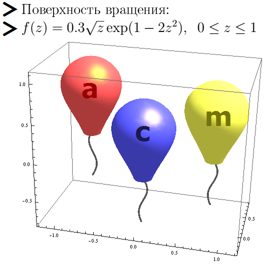
この図は、ある機能の回転面として得られたボールを示しています。
コード
x1 = 0; y1 = 0; z1 = -0.2; x2 = 0.8; y2 = 0.3; z2 = 0; x3 = -0.8; y3 = 0.5; z3 = 0.1; f[z_] := z*(1 - z); f[z_] := 0.3 z^0.5*Exp[1 - 2 z^2]; gz[t_] := -0.6 t; gy[t_] := 0.1 t*(1 - t); gx[t_] := 0.05 Sin[6 t]; Show[ParametricPlot3D[{x1 + f[1 - z]*Cos[phi], y1 + f[1 - z]*Sin[phi], z1 + z}, {z, 0, 1}, {phi, 0, 2*Pi}, PlotStyle -> Directive[Specularity[RGBColor[1, 0.8, 0], 30], Lighter[Blue], Lighting -> {{"Directional", White, {1.5, 0, 3}}, {"Ambient", Darker[White]}}], Mesh -> None], ParametricPlot3D[{x1 + gx[t], y1 + gy[t], z1 + gz[t]}, {t, 0, 1}, PlotStyle -> Directive[Thickness[0.0075], Lighter[Black]]], ParametricPlot3D[{x2 + f[1 - z]*Cos[phi], y2 + f[1 - z]*Sin[phi], z2 + z}, {z, 0, 1}, {phi, 0, 2*Pi}, PlotStyle -> Directive[Specularity[RGBColor[1, 0.8, 0], 30], Lighter[Yellow], Lighting -> {{"Directional", White, {1.5, 0, 3}}, {"Ambient", Darker[White]}}], Mesh -> None], ParametricPlot3D[{x3 + f[1 - z]*Cos[phi], y3 + f[1 - z]*Sin[phi], z3 + z}, {z, 0, 1}, {phi, 0, 2*Pi}, PlotStyle -> Directive[Specularity[RGBColor[1, 0.8, 0], 30], Lighter[Red], Lighting -> {{"Directional", White, {1.5, 0, 3}}, {"Ambient", Darker[White]}}], Mesh -> None], ParametricPlot3D[{x2 + gx[1 - t], y2 + gy[1 - t], z2 + gz[1 - t]}, {t, 0, 1}, PlotStyle -> Directive[Thickness[0.0075], Lighter[Black]]], ParametricPlot3D[{x3 + gx[t], y3 + gy[1 - t], z3 + gz[1 - t]}, {t, 0, 1}, PlotStyle -> Directive[Thickness[0.0075], Lighter[Black]]], PlotRange -> All]
この図は、秋に行われる準々決勝のACMプログラミングの世界チーム選手権を思い起こさせます。 (このチャンピオンシップの決勝戦では、チームには正しく解決された問題に対するボールが与えられます。)
今、私はいくつかの休日の図面を与えます。
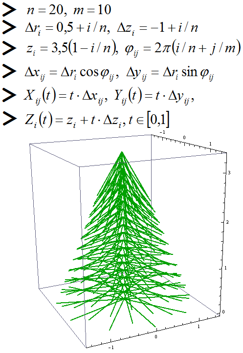
これは新年のために作られた絵です。 これは、セグメントの助けを借りて構築されたクリスマスツリーです。
コード
a = 1; b = 0.5; c = 1.5; h = 3.5; dr[k_] := b + (c - b)/n*k; dz[k_] := -(a - a/n*k); z[k_] := h - h*k/n; cnt = 0; Do[Do[cnt = cnt + 1; phi = j*2*Pi/m + i*2*Pi/n; ldx[cnt] = dr[i]*Cos[phi]; ldy[cnt] = dr[i]*Sin[phi]; ldz[cnt] = dz[i]; lz[cnt] = z[i], {j, 1, m}], {i, 1, n}] ParametricPlot3D[ Table[{ldx[i]*t, ldy[i]*t, lz[i] + ldz[i]*t}, {i, 1, cnt}], {t, 0, 1}, PlotStyle -> Directive[Darker[Green], Thickness[0.005]]
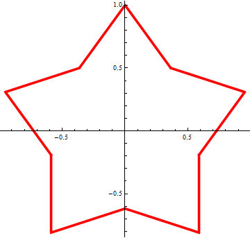
これは2月23日に作られた星です。
コード
gamma = Pi/10; rho = 1; p = rho*Sin[gamma]; k[phi_] := Floor[(phi + 0.2*Pi)/(0.4*Pi)]; s[phi_] := Sign[phi - 0.4*k[phi]*Pi]; alpha[phi_] := s[phi]*(Pi/2 - gamma) + 0.4*k[phi]*Pi; PolarPlot[p/Cos[phi - Pi/2 - alpha[phi - Pi/2]], {phi, 0, 2*Pi}, PlotStyle -> Directive[Red, Thickness[0.01]]]
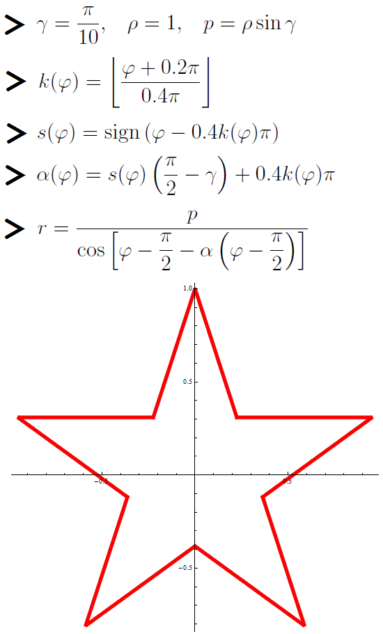
アスタリスクは、線の極座標方程式を使用して設定されます。
ところで、パラメータ
 (星の光線の半分の角度)は変えることができます。 この星は
  。
。
で
 ヒトデに似たアスタリスクが表示されます。
で
 先の尖った星を取得します。

これがバレンタインデーに出てくる写真です。
コード
f[x_, y_] := x^2 + (y - (x^2)^(1/3))^2 - 1; h1[x_] := (x^2)^(1/3) + Sqrt[1 - x^2]; h2[x_] := (x^2)^(1/3) - Sqrt[1 - x^2]; Do[x0[i] = 1 - (i - 1)/6; y0[i] = h1[x0[i]]; k[i] = 4 + i, {i, 1, 6}]; x0[7] = 0; y0[7] = h1[x0[7]]; k[7] = 7; xx0[1] = 0.95; yy0[1] = h2[xx0[1]]; kk[1] = 6; Do[xx0[i] = 1.1 - 0.15*i; yy0[i] = h2[xx0[i]]; kk[i] = 4 + i, {i, 2, 6}] xx0[7] = 0; yy0[7] = h2[xx0[7]]; kk[7] = 6; RegionPlot[ Or @@ Table[(f[(x - x0[i])*k[i], (y - y0[i])*k[i]] <= 0) || (f[(x + x0[i])*k[i], (y - y0[i])*k[i]] <= 0), {i, 1, 7}] || Or @@ Table[(f[(x - xx0[i])*kk[i], (y - yy0[i])*kk[i]] <= 0) || (f[(x + xx0[i])*kk[i], (y - yy0[i])*kk[i]] <= 0), {i, 1, 7}], {x, -1.5, 1.5}, {y, -2.5, 2.5}, PlotStyle -> Red, AspectRatio -> 0.9, PlotRange -> All, MaxRecursion -> 5]

あなたは数学的な認識をすることさえできます:

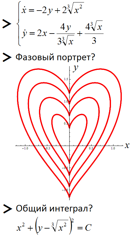
そして、ここにもう一つの数学的な心があります。 1次の2つの微分方程式の自律システムが考慮されます。 このシステムのフェーズポートレートが構築され(システムの軌跡がさまざまな初期条件下で描画されます)、システムの一般的な積分が見つかります。
このシステムは、tに関して一般積分を微分することで取得できます。 このようにして(微分方程式系を解く)、方程式のグラフを作成することができます。
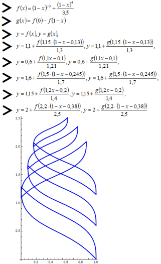
そして、これは3月8日の数学カードです。 この図は、ベルヌーイのレムニスカタのグラフを作成した特定の抽象的なコンピューターを示しています。

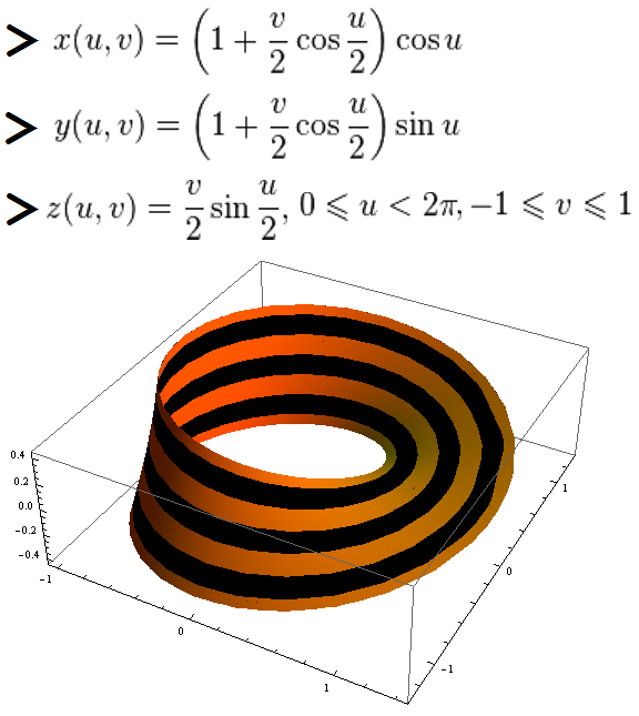
図は、5月9日までにセントジョージメビウスのストリップを示しています。
コード
f[i_, u_] := If[i == 0, -1 + 1/7 + u/7, If[i == 6, -1 + 2*i/7 + u/7, -1 + 2*i/7 + u*2/7]]; ParametricPlot3D[ Evaluate@Table[{(1 + f[i, u]/2*Cos[phi/2])* Cos[phi], (1 + f[i, u]/2*Cos[phi/2])*Sin[phi], f[i, u]/2*Sin[phi/2]}, {i, 0, 6}], {u, 0, 1}, {phi, 0, 2*Pi}, Mesh -> None, PlotStyle -> {Orange, Black, Orange, Black, Orange, Black, Orange}]
次の図は正方形のアカデミックキャップを示しています。この図は9月1日に適しています。
コード
RegionPlot3D[((x^2 + y^2 + (z + 1.75)^2 <= 4 && x^2 + y^2 + (z + 1.75)^2 >= 4 - 1.4) || (z <= 0.1 && z >= 0)) && (z >= -1.5), {x, -2, 2}, {y, -2, 2}, {z, -2, 0.1}, BoxRatios -> {1, 1, 0.8}, PlotStyle -> Blue]

この図は、FEFUロゴを示しています。
ロゴ自体は次のとおりです。

そして、これはFEFUの3Dロゴであり、Wolfram Mathematicaパッケージの数式に従って構築されています。
コード
g[z_] := 1/(1 + (1 - z)^2) - 1/2; h[z_] := 1 - 1/2*Sqrt[1 + (z*Sqrt[3])^2]; f[z_] := If[z >= 0 && z <= 1, g[z], If[z >= 1 && z <= 2, h[z - 1]]] phit[t_] := 2*Pi*t; zt[t_] := 1.4*t; zt1[t_] := 0.3 + 1.4*t; zt2[t_] := 0.6 + 1.4*t; phit1[t_] := 2*Pi*t; phit2[t_] := 2*Pi*t; k = 0.111; ParametricPlot3D[{{f[zt[t] + k*s]*Cos[phit[t]], f[zt[t] + k*s]*Sin[phit[t]], zt[t] + k*s}, {f[zt1[t] + k*s]*Cos[phit1[t]], f[zt1[t] + k*s]*Sin[phit1[t]], zt1[t] + k*s}, {f[zt2[t] + k*s]*Cos[phit2[t]], f[zt2[t] + k*s]*Sin[phit2[t]], zt2[t] + k*s}}, {t, 0, 1}, {s, -1, 1}, PlotStyle -> Blue, Mesh -> None, Axes -> False, Boxed -> False]