退屈なエントリの代わりに
前回は、オペアンプの動作の基本原理を簡単に説明しようとしました。 しかし、トピックを継続するリクエストを拒否することはできません。 今回は、スキームはもう少し複雑ですが、私は退屈な数学的結論を引き伸ばさないようにします。
積分器と微分器
電圧積分を考慮する必要があると想像してください。
したがって、これらの目的のためには、 積分器が必要です。
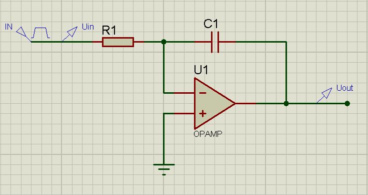
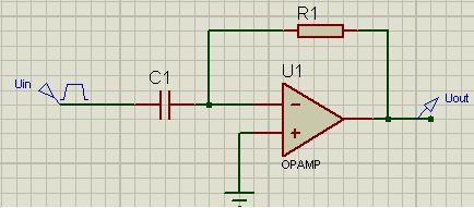
一般的な場合(理想的なオペアンプの場合)、このオプションは考慮されます:
さらに、少し努力することを強くお勧めし、物理学と高等数学の少しのコースを覚えています。 ただし、これは絶対に必要というわけではありません。
コンデンサの充電式を覚えていますか?

料金が時間とともに変化することを考えると、次のことを安全に想定できます。
さらに...非反転入力はグランドに接続されています。 コンデンサの両端の電圧は、出力の反対の電圧に等しい、つまり
 。 つまり、

さらに、解いて統合すると、(ほぼ)最終的な式が得られます。
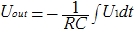
これは、いわば、一般的な用語です。 その結果、時間tの各瞬間に出力電圧が重要な役割を果たすという事実に注意を喚起したいと思います。 私たちはそれを無料の要素として取ります:
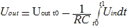
積分は、t0からt1までの時間にわたって発生すると想定するのは論理的です
ここに問題があります。 コンデンサが放電されます。 出力電圧はゼロです。 回路はオフです。 コンデンサの容量は1μFです。 30kオームの抵抗器 入力電圧は最初に-2V、次に2Vです。 極性は毎秒変化します。 つまり、パルスジェネレーターを入力に適用しました。
だから、私たちは決めます。 Proteusで簡単なスキームをまとめる。 グラフを描く。 入力および出力電圧を関数として入力します。 [スケジュールのシミュレーション]をクリックします。 取得するもの:
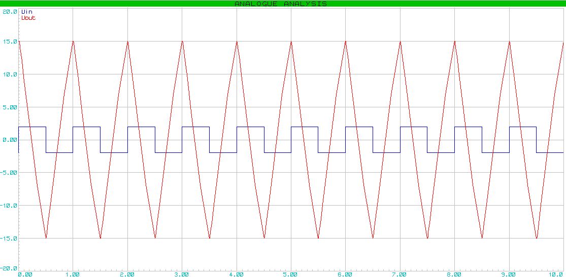
「のこぎり」信号が出ました。 コンデンサは低下の鋭さに影響することに注意してください。 充電/放電する時間があり、放電/放電 *が速すぎないように、合理的な範囲内で変動する必要があります。 ところで、信号がオペアンプの電源内で増幅されると仮定することは論理的です。
次に、 差別化要因に進みます。
インテグレーターほど複雑ではありません。
差別化要因:
そして、これがアナログ計算式です:

そして再び退屈な式...
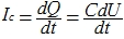
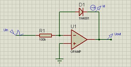
コンデンサを流れる電流は

オペアンプは理想に近いため、コンデンサを流れる電流は抵抗を流れる電流と等しいと仮定できます。
 、つまり、現在の値を代入すると、次のようになります。
前の例のように、より実用的な例を検討してください。 50μFのコンデンサ。 30kオームの抵抗器 入り口で「のこぎり」を提供します。 (正直なところ、プロテウスでは標準的な手段を使用してのこぎりを作ることができなかったので、私はPwlinツールに頼らなければなりませんでした。
その結果、グラフが得られます。

まとめると。
インテグレーター 長方形->のこぎり
差別化要因。 のこぎり->長方形
PS差別化要因と統合要因は、後でまったく異なる形で検討されます。
コンパレータ
コンパレータは、2つの入力電圧を比較するデバイスです。 出力の状態は、どちらの電圧が大きいかに応じて段階的に変化します。 特別なことは何もありません。例を挙げてください。 最初の入力で、3Vに等しい定電圧を供給します。 2番目の入力-振幅が4Vの正弦波信号。 出力から電圧を取り除きます。

グラフには、コメントを必要としない包括的な情報が含まれています。

対数および指数増幅器
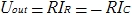
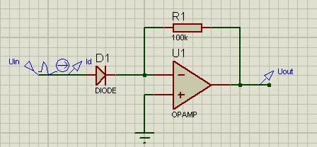
対数特性を得るには、それをもつ要素が必要です。 そのような目的には、ダイオードまたはトランジスタが非常に適しています。 複雑にならないように、ダイオードを使用します。
まず、いつものように、図を示します...
...および式:

eは電子の電荷、Tはケルビン単位の温度、kはボルツマン定数であることに注意してください。
繰り返しますが、物理学コースを覚えておく必要があります。 半導体ダイオードを流れる電流は次のように説明できます。
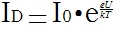 (式の程度が「曲がった」ため、画像はもう少ししました)
ここで、Uはダイオードの電圧です。 I0は、小さな逆バイアスでのリーク電流です。 Prologarithmおよびget:
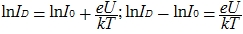
ここから、ダイオードの電圧を取得します(これは出力の電圧と同じです)。

摂氏20度の温度では次のことに注意してください。

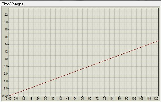
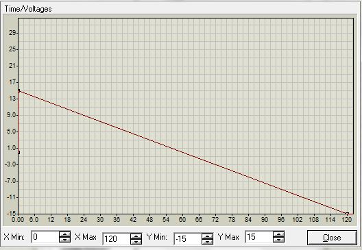
この回路がグラフィカルにどのように機能するかを確認しましょう。 プロテウスを実行します。 入力信号を設定します。
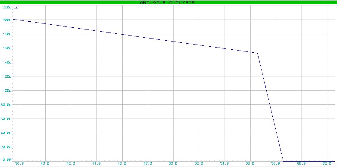
ダイオードの電流は次のように変化します。

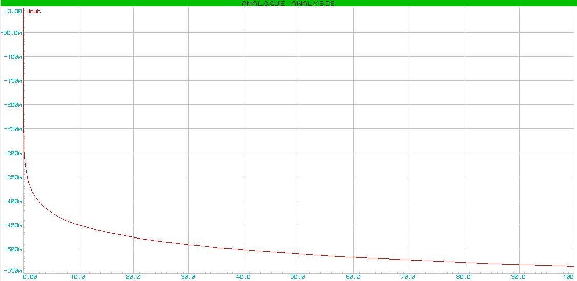
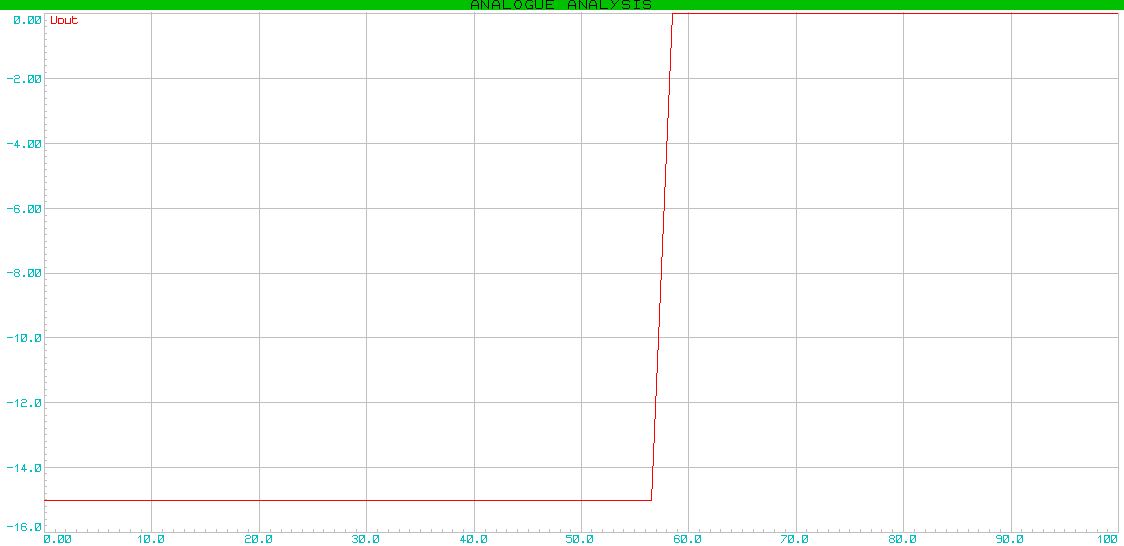
出力電圧は、対数の法則に従って変化します。
次の項目-指数増幅器、私はコメントせずに残します。 ここですべてが明確になることを願っています。
結論の代わりに
このパートでは、数学的結論を最小限に抑え、実用化に焦点を当てようとしました。 楽しんでいただけたでしょうか:-)
* UPD。:コンデンサの充電/放電時間は次のように定義されます:
 どこで
どこで  移行プロセスの時間です。 RC回路の場合、式
  。 Tの間、コンデンサは99%完全に充電/放電されます。 計算に時間が使用される場合があります3