Detailed analysis of the simplex method

Prologue

Recently, there was a need to create a program from scratch that implements the simplex method algorithm. But in the course of the solution, I ran into a problem: there are not so many resources on the Internet where you can look at a detailed theoretical analysis of the algorithm (its rationale: why we take these or those steps) and practical implementation tips - directly, the algorithm. Then I made myself a promise - as soon as I complete the task, I will write my post on this topic. Actually, we’ll talk about this.



Comment. The post will be written in a fairly formal language, but will be provided with comments, which should bring some clarity. Such a format will preserve the scientific approach, and at the same time, it may help some to study this issue.

§one. Statement of the linear programming problem

Definition: Linear programming is a mathematical discipline devoted to the theory and methods of solving extremal problems on sets of n-dimensional space defined by systems of linear equations and inequalities.



The general task of linear programming (hereinafter - LP) has the form:

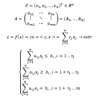
§2. The canonical form of the LP problem

The canonical form of the LP problem:







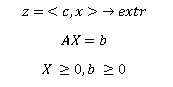
Note: Any LP problem reduces to canonical.



The algorithm for the transition from an arbitrary LP problem to the canonical form:

1. Inequalities with negative $$ $ inline $ b_i $ inline $ multiply by (-1).
2. If an inequality of the form (≤), then add to the left side $$ $ inline $ s_i $ inline $ Is an additional variable, and we obtain equality.
3. If an inequality of the form (≥), then subtract from the left side $$ $ inline $ s_i $ inline $ , and we obtain the equality.
4. We do the replacement of variables:

• If a $$ $ inline $ x_i ≤ 0 $ inline $ then $$ $ inline $ x_i '= -x_i ≥ 0 $ inline $
• If a $$ $ inline $ x_i $ inline $ - any $$ $ inline $ x_i = x_i '- x_i' '$ inline $ where $$ $ inline $ x_i ', x_i''≥ 0 $ inline $

Note: We will number $$ $ inline $ s_i $ inline $ by the inequality number to which we added it.



Comment: $$ $ inline $ s_i $ inline $ ≥0.

§3. Corner points. Basic / free variables. Basic solutions

Definition: Point $$ $ inline $ X ∈ D $ inline $ called a corner point if the representation $$ $ inline $ X = αX ^ 1 + (1-α) X ^ 2, where X ^ 1, X ^ 2 ∈ D; 0 <α <1 $ inline $ only possible with $$ $ inline $ X ^ 1 = X ^ 2 $ inline $ .



In other words, it is impossible to find two points in the region, the interval passing through which contains $$ $ inline $ X $ inline $ (those. $$ $ inline $ X $ inline $ Is not an internal point).



The graphical method for solving the LP problem shows that finding the optimal solution is associated with a corner point. This is the basic concept when developing a simplex method.



Definition: Let there be a system of m equations and n unknowns (m <n). We divide the variables into two sets: (nm) we set the variables equal to zero, and the remaining m variables are determined by solving the system of initial equations. If this solution is unique, then nonzero m variables are called basic; zero (nm) variables - free (non-basic), and the corresponding resulting values ​​of the variables are called the basic solution.

§4. Simplex method

The simplex method allows you to effectively find the optimal solution, avoiding the simple enumeration of all possible corner points. The main principle of the method: the calculations begin with some kind of “starting” basic solution, and then a search is made for solutions that “improve” the value of the objective function. This is possible only if an increase in some variable leads to an increase in the value of the functional.



Prerequisites for applying the simplex method:

1. The task must have a canonical form.
2. The task should have an explicit basis.

Definition: An explicitly selected basis is a vector of the form: $$ $ inline $ (.. 0100 ..) ^ T, (..010 ..) ^ T, (.. 0010 ..) ^ T ... $ inline $ , i.e. only one coordinate of the vector is nonzero and equal to 1.



Note: The base vector has dimension (m * 1), where m is the number of equations in the constraint system.



For convenience of calculations and visualization, simplex tables are usually used:

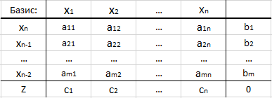
• The first line indicates the "name" of all variables.
• In the first column, the numbers of the basis variables are indicated, and in the last cell, the letter Z (this is the functional line).
• In the "middle of the table" indicate the coefficients of the constraint matrix - aij.
• The last column is the vector of the right-hand sides of the corresponding equations of the constraint system.
• The rightmost cell is the value of the objective function. At the first iteration, it is assumed to be 0.

Note: Basis - variables, coefficients in the matrix of constraints at which form basis vectors.



Note: If the constraints in the original problem are represented by inequalities of the form ≤, then when the problem is reduced to canonical form, the introduced additional variables form the initial basic solution.



Note: The coefficients in the functional line are taken with the “-” sign.



Simplex Method Algorithm:



1. Choose a variable that we will introduce in the basis. This is done in accordance with the principle stated earlier: we must choose a variable whose increase will lead to an increase in the functional. The selection takes place according to the following rule:

• If the task is at a minimum, select the maximum positive element in the last row.
• If the task is at maximum, select the minimum negative.

Such a choice, in fact, corresponds to the principle mentioned above: if the task is at a minimum, then the larger the number we subtract, the faster the functional decreases; for maximum, on the contrary - the larger the number is added, the faster the functional grows.



Note: Although we take the minimum negative number in the problem to the maximum, this coefficient shows the direction of growth of the functional, since the functional line in the simplex table is taken with the “-” sign. A similar situation with minimization.



Definition: The column of the simplex table corresponding to the selected coefficient is called the leading column .



2. Choose a variable that we will introduce in the basis. To do this, you need to determine which of the basis variables is most likely to vanish when the new basis variable grows. Algebraically, this is done as follows:

• The vector of the right-hand parts is divided by the terminating column
• Among the obtained values ​​choose the minimum positive (negative and zero answers are not considered)

Definition: Such a line is called a leading line and corresponds to a variable to be derived from the basis.



Note: In fact, we express the old basis variables from each equation of the constraint system through the rest of the variables and see in which equation the increase in the new basis variable most likely will give 0. Getting into this situation means that we "stumbled" on a new vertex. That is why zero and negative elements are not considered, because obtaining such a result means that the choice of such a new base variable will lead us away from the area beyond which there are no solutions.



3. We are looking for an element standing at the intersection of the leading row and column.



Definition: Such an element is called a leading element .



4. Instead of the variable to be excluded, in the first column (with the names of the base variables), write the name of the variable that we enter into the basis.



5. Next, the process of calculating a new basic solution begins. It occurs using the Jordan-Gauss method .

• New Lead Line = Old Lead Line / Lead
• New row = New row - Row factor in the leading column * New Leading row

Note: A conversion of this kind is aimed at introducing the selected variable into the basis, i.e. representation of the leading column as a base vector.



6. After that, we check the optimality condition. If the resulting solution is not optimal, repeat the whole process again.

§5. Interpretation of the result of the simplex method

1. Optimality



The optimality condition for the resulting solution:

• If the task is at maximum, there are no negative coefficients in the functional row (i.e., with any change in the variables, the value of the resulting functional will not grow).
• If the task is at a minimum, there are no positive coefficients in the functional row (i.e., with any change in the variables, the value of the resulting functional will not decrease).

2. Unlimited functionality



However, it is worth noting that a given functional may not reach a maximum / minimum in a given area. The algebraic attribute of this can be formulated as follows:



When choosing a leading row (excluded variable), the result of termwise division of the vector of the right-hand sides by the leading column contains only zero and negative values.



In fact, this means that no matter what growth we set a new base variable, we will never find a new vertex. So, our function is not limited to the set of feasible solutions.



3. Alternative solutions



When finding the optimal solution, another option is possible - there are alternative solutions (another corner point that gives the same value of the functional).



Algebraic sign of the existence of an alternative:



After reaching the optimal solution, there are zero coefficients for free variables in the functional row.



This means that with the growth of the corresponding variable with a zero coefficient, the value of the functional will not change and a new basic solution will also give the optimum of the functional.

Epilogue

This article is aimed at a deeper understanding of the theoretical part. In the comments and explanations here you can get answers to questions that are usually omitted when studying this method and taken a priori. However, one must understand that many methods of numerical optimization are based on the simplex method (for example, the Gomori method , the M-Method ) and without a fundamental understanding, it is unlikely that much progress will be made in the further study and application of all algorithms of this class.



A little later I will write an article on the practical implementation of the simplex method, as well as several articles on the Method of Artificial Variables (M-Method), the Gomori Method and the Branch and Border Method.



Thanks for attention!



PS



If you are already tormented by the implementation of the simplex method, I advise you to read the book by A. Takh. Introduction to the study of operations - everything is well analyzed there, both in theory and in examples; and also look at examples of solving matburo.ru problems - this will help with implementation in code.