Fractional Brownian motion

Introduction

fBM stands for Fractional Brownian Motion (fractional Brownian motion). But before we start talking about nature, fractals, and procedural reliefs, let's dig into the theory for a moment.



Brownian Motion (BM), simply, without "fragmentation" is a movement in which the position of an object changes with random increments over time (imagine the sequence position+=white_noise();



). From a formal point of view, BM is an integral of white noise. These movements define paths that are random but (statistically) self-similar, i.e. An approximate image of the path resembles the whole path. Fractional Brownian Motion is a similar process in which increments are not completely independent of each other, and there is some kind of memory in this process. If the memory has a positive correlation, then changes in a given direction will tend to future changes in the same direction, and the path will be smoother than with ordinary BM. If the memory has a negative correlation, then a change in the positive direction with a high probability will be followed by a change in the negative, and the path will be much more random. The parameter that controls the behavior of memory or integration, and hence self-similarity, its fractal dimension and power spectrum, is called the Hurst exponent and is usually reduced to H. From a mathematical point of view, H allows us to integrate white noise only partially (say, only 1/3 of integration , hence the "fragmentation" in the name) to create fBM for any desired memory characteristics and appearance. H takes values ​​in the range from 0 to 1, which describe, respectively, a coarse and smooth fBM, and the usual BM is obtained at H = 1/2.









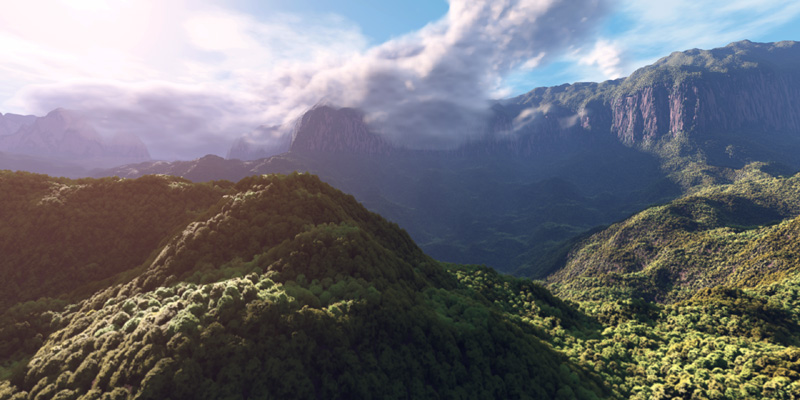
Here, the function fBM () is used to generate topography, clouds, distribution of trees, their color variations and crown details. Rainforest, 2016: https://www.shadertoy.com/view/4ttSWf



All this is very theoretical, and in computer graphics fBM is generated in a completely different way, but I wanted to explain the theory, because it is important to remember it even when you create the graphic. Let's see how this is done in practice:



As we know, self-similar structures, which are random at the same time, are very useful for the procedural modeling of various natural phenomena, from clouds to mountains and textures of the tree bark . It is intuitively clear that figures in nature can be decomposed into several large figures that describe the shape as a whole, a larger number of medium-sized figures that distort the main outline or surface of the original figure, and an even larger number of small figures that add detail to the outline and shape of the previous two. Such an incremental way of adding details to an object, providing us with a simple way to limit the boundaries of frequency ranges for changing LOD (Level Of Detail, levels of detail) and filtering / smoothing shapes, makes it easy to write code and create visually beautiful results. Therefore, it is widely used in films and games. However, I do not think that fBM is well understood by the whole mechanism. In this article, I will describe how it works and how its various spectral and visual characteristics are used for various values ​​of its main parameter H, and I will supplement all this with experiments and measurements.

Basic idea

Usually (there are many ways) fBMs are constructed by calling deterministic and smoothing randomness using the noise function selected by the developer ( value , gradient , cellular , Voronoi , trigonometric, simplex , ..., etc., the chosen option is not very important here), followed by the construction of self-similarity. fBMs are implemented starting from the base noise signal, gradually adding to it smaller and smaller detailed noise calls. Something like this:

 float fbm( in vecN x, in float H ) { float t = 0.0; for( int i=0; i<numOctaves; i++ ) { float f = pow( 2.0, float(i) ); float a = pow( f, -H ); t += a*noise(f*x); } return t; }
      
      

        
        
        
      

    
        
        
        
      
      

        
        
        
      

    
     

This is fBM in its purest form. Each signal (or “wave”) noise (), for which we have “numOctaves,” is additively combined with an intermediate sum, but is compressed horizontally by half, which essentially halves its wavelength, and its amplitude decreases exponentially. Such an accumulation of waves with a coordinated decrease in the wavelength and amplitude creates the self-similarity that we observe in nature. Ultimately, in any given space there is only room for a few big changes, but there is a lot of room for ever smaller changes. Sounds quite reasonable. In fact, such manifestations of the power law are found everywhere in nature.



The first thing you can notice is that the code shown above is not quite similar to most fBM implementations that you could see in Shadertoy and other code examples. The code below is similar to the one shown above, but much more popular, because it does without the costly functions of pow ():

 float fbm( in vecN x, in float H ) { float G = exp2(-H); float f = 1.0; float a = 1.0; float t = 0.0; for( int i=0; i<numOctaves; i++ ) { t += a*noise(f*x); f *= 2.0; a *= G; } return t; }
      
      

        
        
        
      

    
        
        
        
      
      

        
        
        
      

    
     

So, let's start by talking about numOctaves. Since the wavelength of each noise is two times less than the previous one (and the frequency is two times higher), the designation of what should be called “numFrequencies” is replaced by “numOctaves” as a reference to a musical concept: splitting one octave between two notes corresponds doubling the frequency of the base note. In addition, fBM can be created by incrementing the frequency of each noise by an amount different from the two. In this case, the term “octave” will no longer be technically correct, but it is still used. In some cases, it may even be necessary to create waves / noise with frequencies that increase with a constant linear coefficient, and not geometrically, for example, FFT (fast Fourier transform; it can actually be used to generate periodic fBMs (), useful in creating textures ocean). But, as we will see later, most of the basic noise () functions can increase frequencies by magnitudes that are multiples of two, that is, we need very few iterations, and fBMs will still be beautiful. In fact, synthesizing fBM one octave at a time allows us to be very effective - for example, in just 24 octaves / iteration, you can create fBM, covering the entire planet Earth with a detail of 2 meters. If you do this using linearly increasing frequencies, then it will take several orders of magnitude more iterations.



The last note about the sequence of frequencies: if we move from f _i = 2 ⁱ to f _i = 2⋅f _i-1 , then this will give us some flexibility with respect to doubling the frequencies (or reducing by half the wavelengths) - we can easily expand the cycle and change each octave, for example, replacing 2.0 with 2.01, 1.99 and other similar values ​​so that the accumulated zeros and peaks of different noise waves do not overlap each other exactly, which sometimes creates unrealistic patterns. In the case of 2D-fBM, you can also slightly rotate the definition area.



So, in the new software implementation of fBM (), we not only replaced frequency generation from a power-law formulation to an iterative process, but also changed the exponential amplitude (power-law) by geometric series controlled by the “gain” indicator G. It is necessary to perform a transformation from H to G, calculating G = 2 ^-H , which can be easily deduced from the first version of the code. However, more often graphic programmers ignore the Hurst exponent H, or do not even know about it, and work directly with the values ​​of G. Since we know that H varies in the range from 0 to 1, then G varies from 1 to 0.5. And in fact, most programmers set their fBM implementations to a constant value of G = 0.5. Such code will not be as flexible as using the variable G, but there are good reasons for this, and soon we will find out about them.

Self-similarity

As mentioned above, the parameter H determines the self-similarity of the curve. Of course, this is statistical self-similarity. That is, in the case of the one-dimensional fBM (), if we bring the camera horizontally closer to the graph by U, then how much do we need to get closer to the graph vertically by V to get a curve that would look the same? Well, since a = f ^-H , then a⋅V = (f⋅U) ^-H = f ^-H ⋅U ^-H = a⋅U ^-H , that is, V = U ^-H . So, if we bring the camera closer to fBM by a horizontal indicator of 2, then vertically we need to change the scale to 2 ^-H . But 2 ^-H is G! And this is not a coincidence: when using G to scale noise amplitudes, by definition we build self-similarity fBM with a scaling factor G = 2 ^-H .









The Brownian motion (H = 1/2) and the anisotropic zoom are shown on the left. To the right is fBM (H = 1) and isotropic zoom.



Code: https://www.shadertoy.com/view/WsV3zz



What about procedural mountains? The standard Brownian motion has a value of H = 1/2, which gives us G = 0.707107 ... At these values, a curve is generated that looks exactly the same if it is anisotropically scaled along X and Y (if it is a one-dimensional curve). And in fact: for each horizontal zoom factor U, we need to scale the curve vertically by V = sqrt (U), which is not very natural. However, stock market charts very often come close to H = 1/2, because in theory every increment or decrement of the stock value is independent of previous changes (do not forget that BM is a memoryless process). Of course, in practice, certain dependences are present, and these curves are closer to H = 0.6.



But the natural process contains more “memory” in itself, and self-similarity in it is much more isotropic. For example, a higher mountain is wider at its base by the same amount, i.e. mountains usually do not stretch and do not become thinner. Therefore, this makes us understand that for the mountains G should be 1/2 - the same horizontal and vertical zoom. This corresponds to H = 1, i.e. the mountain profiles should be smoother than the stock exchange curve. In fact, it is, and a little later we will measure real profiles to confirm this. But from experience we know that G = 0.5 creates beautiful fractal reliefs and clouds, so G = 0.5 is indeed the most popular G value for all fbm implementations.



But now we have a deeper understanding of H, G and fBM in general. We know that if the value of G is closer to 1, then fBM will be even crazier than pure BM. And in fact: for G = 1, which corresponds to H = 0, we get the noisiest fBM of all.



All these parameterized fBM functions are named, for example, “pink noise” at H = 0, G = 1 or “brown noise” at H = 1/2, G = sqrt (2), which are inherited from the field of digital signal processing (Digital Signal Processing) and are well known to people with sleep problems. Let's dig deeper into the DSP and calculate the spectral characteristics to get a deeper understanding of fBM.

Signal processing perspective

If you think about Fourier analysis, or additive sound synthesis, the implementation of fBM () shown above is similar to the implementation of the Inverse Fourier Transform, which is discrete, like the discrete Fourier transform (DFT), but very sparse and uses a different basic function (in fact it is very different from IFT, but let me explain). In fact, we can generate fBM (), computer graphics and even ocean surfaces using IFFT, but this is quickly becoming a very expensive project. The reason is that IFFT does not additively combine noise waves, but sinusoids, but sinusoids do not very efficiently fill the energy power spectrum, because each sinusoid affects one frequency. However, the noise functions have wide spectra that cover long frequency intervals with a single wave. Both gradient noise and Value noise have such rich and dense graphs of spectral density. Take a look at the graphs:









Sine wave









Value noise









Gradient noise

Note that in the spectrum of both Value noise and gradient noise, the bulk of the energy is concentrated in the lower frequencies, but it is wider - an ideal choice for quickly filling the entire spectrum with several offset and scaled copies. Another sine wave fBM problem is this. that it, of course, generates repeating pattenes, which are most often undesirable, although they can be useful for generating seamless textures. The advantage of fBM () based on sin () is that it is superproductive, because trigonometric functions are performed in iron much faster than building noise using polynomials and hashes / lut, so sometimes it is still worth using fBM based on sine waves from performance considerations, even if poor landscapes are created.



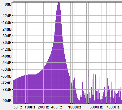
Now let's take a look at the graphs of the density of spectra for fBM with different values ​​of H. Pay particular attention to the marks on the vertical axis, because all three graphs are normalized and do not describe the same slopes, although at first glance they look almost the same. If we denote the negative slope of these spectral graphs as “B”, then since these graphs have a logarithmic scale, the spectrum will follow a power law of the form f ^-B . In this test, I use 10 octaves of normal gradient noise to build the fBM shown below.









G = 1.0 (H = 0)









G = 0.707 (H = 1/2)









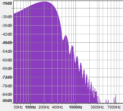
G = 0.5 (H = 1)



As we can see, the energy fBM with H = 0 (G = 1) attenuates at 3 dB per octave, or, in fact, back in value to the frequency. This is a power law f ^-1 (B = 1), which is called “pink noise” and sounds like rain.



fBM () with H = 1/2 (G = 0.707) generates a spectrum that attenuates faster, at 6 dB per octave, that is, it has less high frequencies. It actually sounds deeper, as if you hear rain, but this time from your room with the windows closed. Attenuation of 6 dB / octave means that the energy is proportional to f ^-2 (B = 2), and this is actually a characteristic of Brownian motion in the DSP.



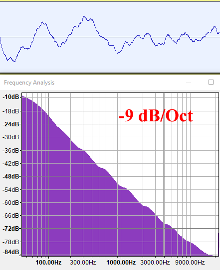
Finally, our favorite fBM from computer graphics with H = 1 (G = 0.5) generates a spectral density graph with a decay of 9 dB / octave, that is, the energy is inversely proportional to the frequency cube (f ^-3 , B = 3). This is a signal with a constantly low frequency, which corresponds to a process with positive correlation memory, which we spoke about at the beginning. This type of signal does not have its own name, so I am tempted to call it “yellow noise” (simply because this name is no longer used for anything). As we know, it is isotropic, which means it simulates a lot of self-repeating natural forms.



In fact, I will confirm my words about the similarity with nature by making the measurements given in the next section of the article.

Title	H	G = 2 -H	B = 2H + 1	dB / oct	Sound
Blue	-	-	+1	+3	Spray water. Link
White	-	-	0	0	Wind in the leaves. Link
Pink	0	one	-one	-3	Rain. Link
Brown	1/2	sqrt (2)	-2	-6	Rain heard from home. Link
Yellow	one	1/2	-3	-9	Engine behind the door

Measurements

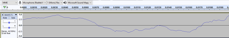
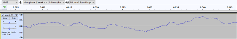
First I must warn you that it will be a very unscientific experiment, but I still want to share it. I took photographs of mountain ranges parallel to the image plane to avoid perspective distortion. Then I divided the images into black and white, and then converted the contact surface of the sky and mountains into a 1D signal. Then I interpreted it as a WAV sound file and calculated its frequency graph, as is the case with the synthetic fBM () signals that I analyzed above. I selected images with a sufficiently large resolution so that the FFT algorithm had significant data for work.









Source: Greek Reporter









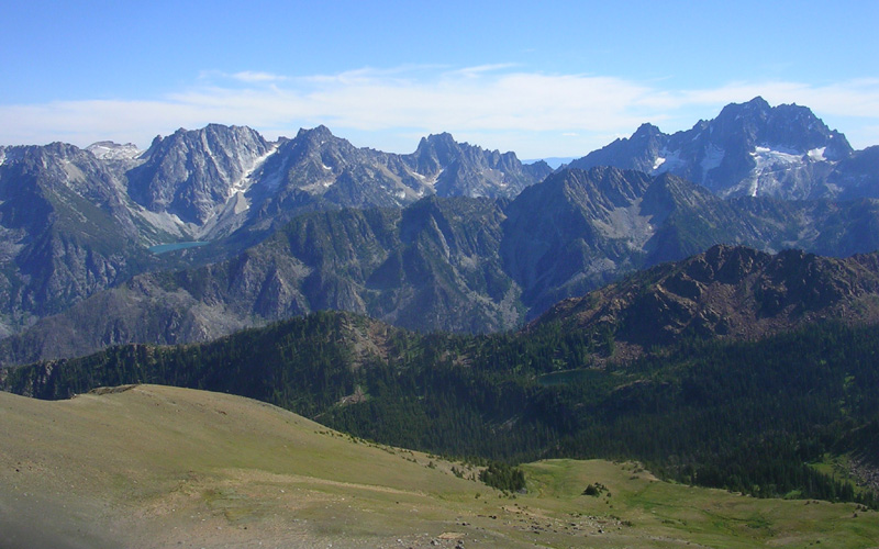
Source: Wikipedia







































It seems that the results really indicate that the mountain profiles follow a frequency distribution of -9 dB / octave, which corresponds to B = -3 or H = 1 or G = 0.5, or, in other words, yellow noise.



Of course, the experiment was not rigorous, but it confirms our intuitive understanding and what we already know from experience and work with computer graphics. But I hope now we have begun to understand this better!