Discrete Math for WMS: Clustering Stock Lots

The article describes how, when implementing a WMS- system, we were faced with the need to solve a non-standard clustering problem and with what algorithms we solved it. We’ll tell you how we applied a systematic, scientific approach to solving the problem, what difficulties we encountered and what lessons we learned.



This publication begins a series of articles in which we share our successful experience in implementing optimization algorithms in warehouse processes. The aim of the series of articles is to acquaint the audience with the types of tasks of optimizing warehouse operations that arise in almost any medium and large warehouse, as well as tell about our experience in solving such problems and the pitfalls encountered along this way. The articles will be useful to those who work in the warehouse logistics industry, implement WMS systems, as well as programmers who are interested in mathematics applications in business and process optimization in the enterprise.

Process bottleneck

In 2018, we made a project to introduce a WMS system at the warehouse of the LD Trading House company in Chelyabinsk. Introduced the product “1C-Logistics: Warehouse Management 3” for 20 jobs: WMS operators, storekeepers, forklift drivers. Warehouse average of about 4 thousand m2, the number of cells 5000 and the number of SKU 4500. The warehouse stores ball valves of their own production in different sizes from 1 kg to 400 kg. Inventories are stored in the context of batches due to the need to select goods according to FIFO and the "in-line" specifics of product placement (explanation below).



When designing automation schemes for warehouse processes, we were faced with the existing problem of non-optimal storage of stocks. Stacking and storage of cranes has, as we have already said, “in-line” specifics. That is, the products in the cell are stacked in rows one on top of the other, and the ability to put a piece on a piece is often absent (they simply fall, and the weight is not small). Because of this, it turns out that only one nomenclature of one batch can be in one piece storage unit;



Products arrive at the warehouse daily and each arrival is a separate batch. In total, as a result of 1 month of warehouse operation, 30 separate lots are created, despite the fact that each should be stored in a separate cell. The goods are often taken not in whole pallets, but in pieces, and as a result, in the piece selection area, in many cells the following picture is observed: in a cell with a volume of more than 1 m3 there are several pieces of cranes that occupy less than 5-10% of the cell volume (see Fig. 1 )







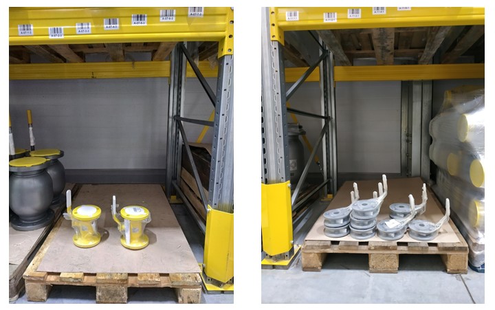
Fig 1. Photo of several pieces of goods in a cell



On the face of the suboptimal use of storage capacity. To imagine the scale of the disaster, I can cite the figures: on average there are between 100 and 300 cells of such cells with a "scanty" residue in different periods of the warehouse’s operation. Since the warehouse is relatively small, in the loading seasons of the warehouse this factor becomes a “narrow neck” and greatly inhibits warehouse processes.

Idea of ​​solving a problem

The idea came up: to bring the balances with the closest dates to one single lot and place such balances with a unified batch compactly together in one cell, or in several if there isn’t enough space in one to accommodate the total number of balances.





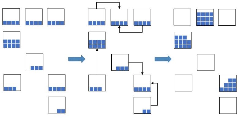
Fig. 2. Cell compression scheme



This allows you to significantly reduce the occupied warehouse space, which will be used for the newly placed goods. In the situation of overloading warehouse capacities, such a measure is extremely necessary, otherwise there may simply not be enough free space for the placement of new goods, which will lead to a stop in the warehouse processes of placement and replenishment. Previously, before the implementation of the WMS- system, such an operation was performed manually, which was not effective, since the process of finding suitable residues in the cells was quite long. Now, with the introduction of WMS systems, they decided to automate the process, speed it up and make it intelligent.



The process of solving this problem is divided into 2 stages:

• at the first stage we find groups of parties close in date for compression;
• at the second stage, for each group of batches we calculate the most compact placement of product residues in cells.

In the current article, we will focus on the first stage of the algorithm, and leave the coverage of the second stage for the next article.

Search for a mathematical model of a problem

Before we sit down to write code and invent our bicycle, we decided to approach this problem scientifically, namely: formulate it mathematically, reduce it to the well-known discrete optimization problem and use effective existing algorithms to solve it, or take these existing algorithms as a basis and modify them under the specifics of the practical task to be solved.



Since it clearly follows from the business statement of the problem that we are dealing with sets, we formulate such a problem in terms of set theory.



Let be $$$P$ - the set of all batches of residues of a certain product in stock. Let be $$$C$ - the given constant of days. Let be $$$K$ - a subset of batches where the date difference for all pairs of batches of the subset does not exceed the constant $$$C$ . Find the minimum number of disjoint subsets $$$K$ such that all subsets $$$K$ collectively would give a lot $$$P$ .



Moreover, we need to find not just the minimum number of subsets, but so that such subsets would be as large as possible. This is due to the fact that after the clustering of batches, we will “compress” the remains of the batches found in the cells. Let us illustrate with an example. Suppose there are many parties distributed on the time axis, as in Figure 3.





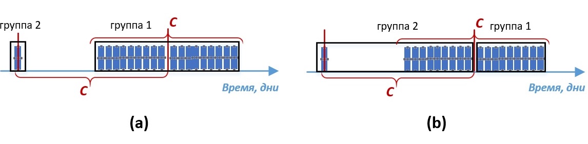
Fig. 3. Variants of splitting multiple batches



Of the two options for splitting the set P with the same number of subsets, the first partition (a) is most beneficial for our task. Since, the more parties will be in groups, the more compression combinations appear, and thus the more likely to find the most compact compression. Of course, such a rule is nothing more than a heuristic and our speculative assumption. Although, as a computational experiment showed, if such a maximization condition is taken into account, the compactness of the subsequent compression of the residuals becomes on average 5–10% higher than the compression that was constructed without taking into account such a condition.



In other words, in short, we need to find groups or clusters of similar parties where the criterion of similarity is determined by a constant $$$C$ . This task reminds us of the well-known clustering problem. It is important to say that the problem under consideration differs from the clustering problem in that in our problem there is a strictly specified condition for the criterion of similarity of cluster elements, determined by the constant $$$C$ , and in the clustering problem there is no such condition. The statement of the clustering problem and information on this task can be found here.



So, we managed to formulate the problem and find the classical problem with a similar formulation. Now it is necessary to consider well-known algorithms for its solution, so as not to reinvent the wheel, but to take the best practices and apply them. To solve the clustering problem, we considered the most popular algorithms, namely: $$$k$ -means $$$c$ -means, algorithm for selecting connected components, minimal spanning tree algorithm. A description and analysis of such algorithms can be found here.



To solve our problem, clustering algorithms $$$k$ -means and $$$c$ -means are not applicable at all, since the number of clusters is never known beforehand $$$k$ and such algorithms do not take into account the limitation of the constant of days. Such algorithms were initially discarded.

To solve our problem, the algorithm for selecting connected components and the minimum spanning tree algorithm are more suitable, but, as it turned out, they cannot be applied “head on” to the problem being solved and get a good solution. To clarify this, we consider the logic of the operation of such algorithms as applied to our problem.



Consider the graph $$$G$ in which the tops are a lot of parties $$$P$ , and the edge between the vertices $$$p_1$ and $$$p_2$ has a weight equal to the difference of days between batches $$$p_1$ and $$$p_2$ . In the algorithm for selecting connected components, an input parameter is specified $$$R$ where $$$R \ leq C$ , and in the graph $$$G$ all edges for which weight is removed are removed $$$R$ . Only the closest pairs of objects remain connected. The meaning of the algorithm is to select such a value $$$R$ in which the graph “falls apart” into several connected components, where the parties belonging to these components satisfy our similarity criterion, which is determined by the constant $$$C$ . The resulting components are clusters.



The minimum spanning tree algorithm first builds on a graph $$$G$ minimal spanning tree, and then sequentially removes the edges with the highest weight until the graph “falls apart” into several connected components, where the lots belonging to these components will also satisfy our similarity criterion. The resulting components will be clusters.



When using such algorithms to solve the problem under consideration, a situation may arise as in Figure 4.





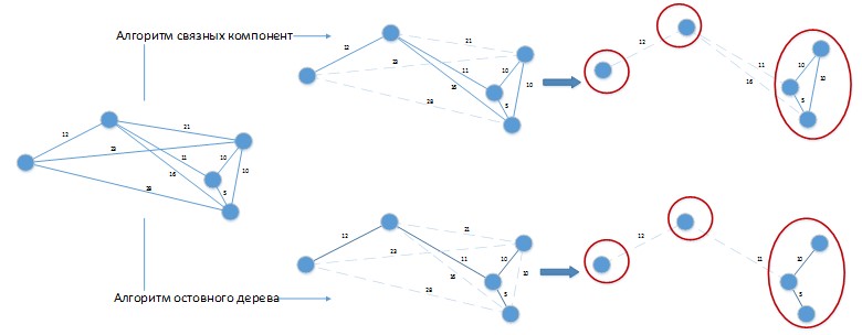
Figure 4. Application of clustering algorithms to the problem being solved.



Suppose we have a constant difference of the days of the parties is 20 days. Graph $$$G$ was depicted in a spatial form for the convenience of visual perception. Both algorithms gave a solution with 3 clusters, which can be easily improved by combining batches placed in separate clusters among themselves! Obviously, such algorithms need to be further developed according to the specifics of the problem being solved and their pure application to the solution of our problem will give poor results.









So, before starting to write the code of graph algorithms modified for our task and reinventing our bicycle (the silhouettes of the square wheels were already guessed in its silhouettes), we again decided to approach this problem scientifically, namely: try to reduce it to another discrete problem optimization, in the hope that existing algorithms for its solution can be applied without modifications.



The next search for a similar classic problem was successful! It was possible to find a discrete optimization problem, the statement of which almost 1 in 1 coincides with the statement of our problem. This problem turned out to be the problem of covering the set . We present the statement of the problem as applied to our specifics.



There is a finite set $$$P$ and family $$$S$ of all its disjoint subsets of parties, such that the date difference for all pairs of parties of each subset $$$I$ from the family $$$S$ does not exceed constants $$$C$ . Coating is called a family $$$U$ least power whose elements belong $$$S$ such that the union of sets $$$I$ from the family $$$U$ should give a lot of all the parties $$$P$ .



A detailed analysis of this problem can be found here and here. Other options for the practical application of the coverage problem and its modifications can be found here.



The only slight difference between the considered problem and the classical problem of covering the set is the need to maximize the number of elements in the subsets. Of course, one could look for articles in which such a special case was considered and, most likely, they would be found. But, from the next search for articles, we were saved by the fact that the well-known "greedy" algorithm for solving the classical problem of covering a set builds a partition just taking into account the maximization of the number of elements in the subsets. So, we ran a little ahead, and now everything is in order.

The algorithm for solving the problem

We decided on the mathematical model of the problem to be solved. Now we begin to consider the algorithm for its solution. Subsets $$$I$ from the family $$$S$ can be easily found, for example, by such a procedure.

1. Step 0. Arrange batches from the set $$$P$ in ascending order of their dates. We believe that all parties are not marked as viewed.
2. Step 1. Find the party with the smallest date from the parties not yet viewed.
3. Step 2. For the found party, moving to the right, we include in the subset $$$I$ all parties whose dates differ from the current one by no more than $$$C$ days. All lots included in the set $$$I$ mark as viewed.
4. Step 3. If, when moving to the right, the next batch cannot be included in $$$I$ , then go to step 1.

The problem of covering a set is $$$NP$ - difficult, which means that for its solution there is no fast (with an operating time equal to a polynomial from the input data) and accurate algorithm. Therefore, to solve the problem of covering the set, a fast greedy algorithm was chosen, which of course is not exact, but has the following advantages:

• For problems of small dimension (and this is just our case), it computes solutions that are close enough to optimum. As the size of the problem grows, the quality of the solution deteriorates, but still rather slowly;
• Very easy to implement;
• Fast, since the estimate of its operating time is $$$O (mn)$ .

The greedy algorithm selects sets guided by the following rule: at each stage, a set is selected that covers the maximum number of elements not yet covered. A detailed description of the algorithm and its pseudo-code can be found here. The implementation of the algorithm in 1C language in the spoiler is lower (about why they began to implement it in the "yellow" language in the next chapter).





Of course, the optimality of such an algorithm is out of the question - heuristics, to say nothing. You can come up with such examples on which such an algorithm would be wrong. Such errors arise when, at some iteration, we find several sets with the same number of elements and select the first one that comes up, because the strategy is greedy: I ​​took the first thing that caught my eye and the “greedy” was satisfied.



It may well be that such a choice may lead to suboptimal results at subsequent iterations. But the accuracy of such a simple algorithm is still pretty good in most cases. If you want to get the solution to the problem more accurately, then you need to use more complex algorithms, for example, as in work : a probabilistic greedy algorithm, an ant colony algorithm, etc. The results of comparing such algorithms on the generated random data can be found in the work.

Implementation and implementation of the algorithm

Such an algorithm was implemented in 1C language and was included in an external processing called “Compression of residues”, which was connected to the WMS- system. We did not implement the algorithm in C ++ and use it from an external Native component, which would be more correct, since the speed of C ++ code is several times and in some examples even ten times faster than the speed of similar code in 1C . In 1C, the algorithm was implemented to save development time and ease of debugging on the customer’s working base. The result of the algorithm is shown in Figure 6.





Fig. 6. Residue Compression Processing



Figure 6 shows that in the indicated warehouse the current stock of goods in storage cells was divided into clusters, inside which the dates of consignments differ by no more than 30 days. Since the customer manufactures and stores metal ball valves with a shelf life of several years, this date difference can be neglected. Note that currently such processing is used in production systematically, and WMS operators confirm the good quality of batch clustering.

Conclusions and continued

The main experience that we obtained from solving such a practical problem is to confirm the effectiveness of using the paradigm: Mat. task statement $$$\ rightarrow$ famous mat. model $$$\ rightarrow$ famous algorithm $$$\ rightarrow$ algorithm taking into account the specifics of the task. There are already more than 300 years of discrete optimization, and during this time people managed to consider a lot of problems and gain a lot of experience in solving them. First of all, it is more advisable to turn to this experience, and only then begin to reinvent your bicycle.



It is also important to say that the solution to the clustering problem could be considered not separately from the solution to the problem of compressing the remainder of the parties, but to solve such problems together. That is, to select such a partition of parties into clusters that would give the best compression. But the solution to such problems was decided to be divided for the following reasons:

• Limited budget for algorithm development. The development of such a general, and therefore more complex algorithm would be more time consuming.
• The complexity of debugging and testing. The general algorithm would be more difficult to test and debug at the acceptance stage, and bugs in it would be more difficult and longer to debug in real-time mode. For example, an error occurred and it is not clear where to dig: roofing felts towards clustering, roofing felts towards compression?
• Transparency and manageability. Separation of the two tasks makes the compression process more transparent, and therefore more manageable for end users - WMS operators. They can remove some cells from compression or edit the compressible quantity for some reason.

In the next article, we will continue the discussion of optimization algorithms and consider the most interesting and much more complex: the optimal algorithm for the “compression” of residuals in cells, which uses input from the batch clustering algorithm as input.



Prepared an article

Roman Shangin, Programmer, Project Department,

First BIT company, Chelyabinsk