Neural networks and deep learning, chapter 5: why are deep neural networks so hard to train?

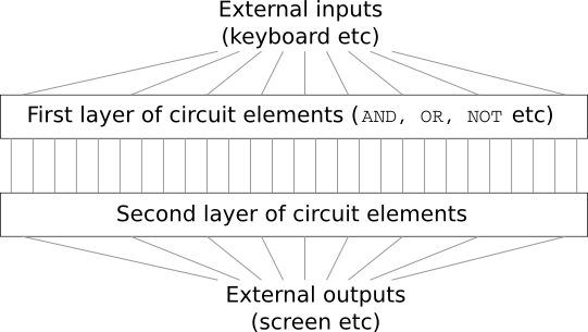
Imagine that you are an engineer, and you were asked to develop a computer from scratch. Once you are sitting in the office, you are struggling to design logical circuits, distribute the AND, OR valves, and so on - and suddenly your boss comes in and tells you the bad news. The client just decided to add an unexpected requirement to the project: the scheme of the entire computer should have no more than two layers:







You are amazed and tell the boss: “Yes, the client is crazy!”



The boss replies: “I think so too. But the client must get what he wants. "



In fact, in a narrow sense, the client is not completely insane. Suppose you are allowed to use a special logic gate that allows you to connect any number of inputs via AND. And you are allowed to use the NAND gate with any number of inputs, that is, such a gate that adds up a lot of inputs through AND, and then reverses the result. It turns out that with such special valves you can calculate any function with just a two-layer circuit.



However, just because something can be done does not mean that it is worth doing. In practice, when solving problems associated with the design of logic circuits (and almost all algorithmic problems), we usually start by solving subproblems, and then gradually assemble a complete solution. In other words, we build a solution through many levels of abstraction.



For example, suppose we design a logic circuit for multiplying two numbers. It is likely that we will want to build it from subcircuits that implement operations such as the addition of two numbers. Addition subcircuits, in turn, will consist of subcircuits adding two bits. Roughly speaking, our scheme will look like this:







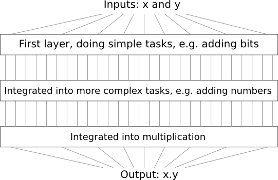
That is, the last circuit contains at least three layers of circuit elements. In fact, there are likely to be more than three layers in it when we break up the subtasks into smaller ones than those that I described. But you understood the principle.



Therefore, deep schemes facilitate the design process. But they help not only in the design. There is mathematical evidence that to calculate some functions in very shallow circuits it is required to use an exponentially greater number of elements than in deep ones. For example, there is a famous series of scientific works of the 1980s, where it was shown that calculating the parity of a set of bits requires an exponentially larger number of gates with a shallow circuit. On the other hand, when using deep schemes, it is easier to calculate the parity using a small scheme: you simply calculate the parity of the pairs of bits, and then use the result to calculate the parity of the pairs of bits, and so on, quickly reaching the general parity. Therefore, deep schemes can be much more powerful than shallow ones.



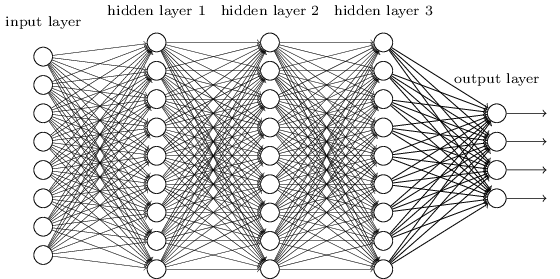
So far, this book has used an approach to neural networks (NS), similar to the requests of a crazy client. Almost all the networks we worked with had a single hidden layer of neurons (plus the input and output layers):







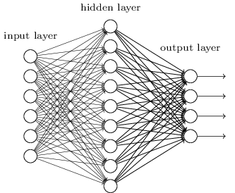
These simple networks turned out to be very useful: in previous chapters we used such networks to classify handwritten numbers with an accuracy exceeding 98%! However, it is intuitively clear that networks with many hidden layers will be much more powerful:







Such networks can use intermediate layers to create many levels of abstraction, as is the case with our Boolean schemes. For example, in the case of pattern recognition, neurons of the first layer can learn to recognize faces, neurons of the second layer - more complex shapes, for example, triangles or rectangles created from faces. Then the third layer will be able to recognize even more complex shapes. And so on. It is likely that these many layers of abstraction will give deep networks a compelling advantage in solving problems of recognizing complex patterns. Moreover, as in the case of circuits, there are theoretical results confirming that deep networks inherently have more capabilities than shallow ones.



How do we train these deep neural networks (GNSs)? In this chapter, we will try to train STS using our workhorse among the training algorithms - stochastic gradient backward propagation descent. However, we will encounter a problem - our GNS will not work much better (if at all surpassed) than shallow ones.



This failure seems strange in the light of the discussion above. But instead of giving up on the STS, we will delve deeper into the problem and try to understand why the STS is hard to train. When we take a closer look at the issue, we will find that different layers in the STS learn at very different speeds. In particular, when the last layers of the network are trained well, the first often get stuck during training, and learn almost nothing. And it's not just bad luck. We will find fundamental reasons for slowing down learning that are associated with the use of gradient-based learning techniques.



Burrowing deeper into this problem, we learn that the reverse phenomenon may also occur: the early layers can learn well, and the later ones can get stuck. In fact, we will discover the internal instability associated with gradient descent training in deep multilayer NSs. And because of this instability, either the early or late layers often get stuck in training.



All this sounds pretty unpleasant. But plunged into these difficulties, we can begin to develop ideas on what needs to be done for effective training of STS. Therefore, these studies will be a good preparation for the next chapter, where we will use deep learning to approach the problems of image recognition.

Fading gradient problem

So what goes wrong when we try to train a deep network?



To answer this question, we return to the network containing only one hidden layer. As usual, we will use the MNIST digit classification problem as a sandbox for training and experimentation.



If you want to repeat all these steps on your computer, you must have Python 2.7 installed, the Numpy library, and a copy of the code that can be taken from the repository:

git clone https://github.com/mnielsen/neural-networks-and-deep-learning.git
      
      

        
        
        
      

    
        
        
        
      
      

        
        
        
      

    
     

You can do without git by simply downloading data and code . Go to the src subdirectory and from the python shell load the MNIST data:

 >>> import mnist_loader >>> training_data, validation_data, test_data = \ ... mnist_loader.load_data_wrapper()
      
      

        
        
        
      

    
        
        
        
      
      

        
        
        
      

    
     

Configure the network:

 >>> import network2 >>> net = network2.Network([784, 30, 10])
      
      

        
        
        
      

    
        
        
        
      
      

        
        
        
      

    
     

Such a network has 784 neurons in the input layer, corresponding to 28 × 28 = 784 pixels of the input image. We use 30 hidden neurons and 10 weekends, corresponding to ten possible classification options for the numbers MNIST ('0', '1', '2', ..., '9').



Let's try to train our network for 30 whole epochs using mini-packages of 10 training examples at a time, learning speed η = 0.1 and regularization parameter λ = 5.0. During training, we will track the accuracy of the classification through validation_data:

 >>> net.SGD(training_data, 30, 10, 0.1, lmbda=5.0, ... evaluation_data=validation_data, monitor_evaluation_accuracy=True)
      
      

        
        
        
      

    
        
        
        
      
      

        
        
        
      

    
     

We get a classification accuracy of 96.48% (or so - the numbers will vary with different launches), comparable to our earlier results with similar settings.



Let's add another hidden layer, also containing 30 neurons, and try to train the network with the same hyperparameters:

 >>> net = network2.Network([784, 30, 30, 10]) >>> net.SGD(training_data, 30, 10, 0.1, lmbda=5.0, ... evaluation_data=validation_data, monitor_evaluation_accuracy=True)
      
      

        
        
        
      

    
        
        
        
      
      

        
        
        
      

    
     

Classification accuracy improves to 96.90%. It is inspiring - a slight increase in depth helps. Let's add another hidden layer of 30 neurons:

 >>> net = network2.Network([784, 30, 30, 30, 10]) >>> net.SGD(training_data, 30, 10, 0.1, lmbda=5.0, ... evaluation_data=validation_data, monitor_evaluation_accuracy=True)
      
      

        
        
        
      

    
        
        
        
      
      

        
        
        
      

    
     

It didn’t help. The result even fell to 96.57%, a value close to the original shallow network. And if we add another hidden layer:

 >>> net = network2.Network([784, 30, 30, 30, 30, 10]) >>> net.SGD(training_data, 30, 10, 0.1, lmbda=5.0, ... evaluation_data=validation_data, monitor_evaluation_accuracy=True)
      
      

        
        
        
      

    
        
        
        
      
      

        
        
        
      

    
     

Then the classification accuracy will again fall, already to 96.53%. Statistically, this drop is probably insignificant, but there is nothing good about it.



This behavior seems strange. It seems intuitively that additional hidden layers should help the network learn more complex classification functions, and better cope with the task. Of course, the result should not worsen, because in the worst case, additional layers simply will not do anything. However, this does not happen.



So what is going on? Let's assume that additional hidden layers can help in principle, and that the problem is that our training algorithm does not find the correct values ​​for weights and offsets. We would like to understand what is wrong with our algorithm, and how to improve it.



To understand what went wrong, let's visualize the network learning process. Below I built a part of the network [784,30,30,10], in which there are two hidden layers, each of which has 30 hidden neurons. On the diagram, each neuron has a bar indicating the rate of change in the process of learning the network. A large bar means that the weights and displacements of the neuron change quickly, and a small one means that they change slowly. More precisely, the bar denotes the ∂C / ∂b gradient of the neuron, that is, the rate of change of value with respect to the displacement. In Chapter 2, we saw that this gradient value controls not only the rate of change of displacement during training, but also the rate of change of input neuron weights. Do not worry if you cannot recall these details: you just need to keep in mind that these bars indicate how quickly the weights and displacements of the neurons change during network learning.



To simplify the diagram, I drew only six of the upper neurons in two hidden layers. I lowered the incoming neurons because they have no weights or biases. I omitted output neurons as well, since we are comparing two layers, and it makes sense to compare layers with the same number of neurons. The diagram was built using the generate_gradient.py program at the very beginning of training, that is, immediately after the network was initialized.







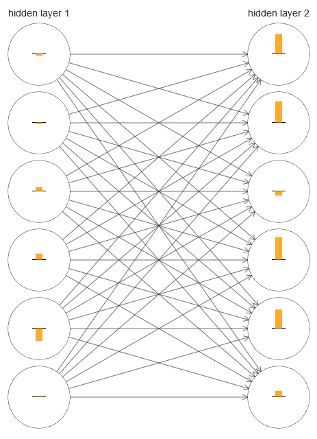
The network was initialized by chance, so this diversity in the speed of training of neurons is not surprising. However, it immediately catches the eye that in the second hidden layer the strips are basically much more than in the first. As a result, neurons in the second layer will learn much faster than in the first. Is this a coincidence, or are neurons in the second layer likely to learn faster than neurons in the first?



To know exactly, it will be good to have a general way of comparing the learning speed in the first and second hidden layers. To do this, let us denote the gradient as δ ^l _j = ∂C / ∂b ^l _j , that is, as the gradient of neuron No. j in the layer No. l. In the second chapter, we called it a “mistake”, but here I will informally call it a “gradient”. Informally - since this value does not include explicitly partial derivatives of the cost by weight, ∂C / ∂w. The gradient δ ¹ can be thought of as a vector whose elements determine how quickly the first hidden layer learns, and δ ² as a vector whose elements determine how quickly the second hidden layer learns. We use the lengths of these vectors as approximate estimates of the learning speed of the layers. That is, for example, the length || δ ¹ || measures the learning speed of the first hidden layer, and the length || δ ² || measures the learning speed of the second hidden layer.



With these definitions and the same configuration as above, we find that || δ ¹ || = 0.07, and || δ ² || = 0.31. This confirms our suspicions: the neurons in the second hidden layer learn much faster than the neurons in the first hidden layer.



What happens if we add more hidden layers? With three hidden layers in the network [784,30,30,30,10] the corresponding learning speeds will be 0.012, 0.060 and 0.283. Again, the first hidden layers learn much slower than the last. Add another hidden layer with 30 neurons. In this case, the corresponding learning speeds will be 0.003, 0.017, 0.070 and 0.285. The pattern is preserved: the early layers learn more slowly than the later ones.



We studied the speed of learning at the very beginning - immediately after the initialization of the network. How does this speed change as you learn? Let's go back and look at the network with two hidden layers. The speed of learning changes in it like this:







To get these results, I used batch gradient descent with 1000 training images and training for 500 eras. This is slightly different from our usual procedures - I did not use mini-packages and took only 1000 training images, instead of a full set of 50,000 pieces. I'm not trying to trick and deceive you, but it turns out that using stochastic gradient descent with mini-packets brings a lot more noise to the results (but if you average the noise, the results are similar). Using the parameters I have chosen, it is easy to smooth the results so that we can see what is happening.



In any case, as we see, two layers begin training at two very different speeds (which we already know). Then the speed of both layers drops very quickly, after which a rebound occurs. However, all this time, the first hidden layer learns much slower than the second.



What about more complex networks? Here are the results of a similar experiment, but with a network with three hidden layers [784,30,30,30,10]:







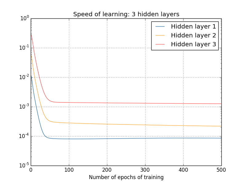
And again, the first hidden layers learn much slower than the last. Finally, let's try to add a fourth hidden layer (network [784,30,30,30,30,10]), and see what happens when it is trained:







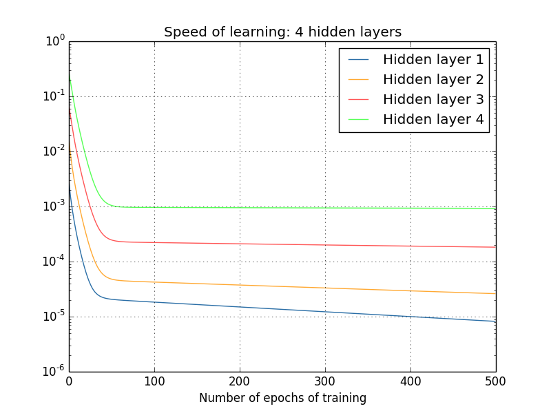
And again, the first hidden layers learn much slower than the last. In this case, the first hidden layer learns about 100 times slower than the last. No wonder we had such problems learning these networks!



We made an important observation: at least in some GNSs, the gradient decreases when moving in the opposite direction along hidden layers. That is, the neurons in the first layers are trained much more slowly than the neurons in the last. And although we observed this effect in only one network, there are fundamental reasons why this happens in many NSs. This phenomenon is known as the “vanishing gradient problem” (see works 1 , 2 ).



Why is there a fading gradient problem? Are there any ways to avoid it? How do we deal with it when training STS? In fact, we will soon find out that it is not inevitable, although the alternative does not look very attractive to her: sometimes in the first layers the gradient is much larger! This is already a problem of explosive gradient growth, and it is no more good in it than in the problem of a disappearing gradient. In general, it turns out that the gradient in the STS is unstable, and is prone to either explosive growth or to disappear in the first layers. This instability is a fundamental problem for gradient GNS training. This is what we need to understand, and possibly solve it somehow.



One of the reactions to a fading (or unstable) gradient is to think about whether this is actually a serious problem? Let us briefly distract from the NS, and imagine that we are trying to numerically minimize the function f (x) from one variable. Wouldn't it be great if the derivative f ′ (x) was small? Would this not mean that we are already close to the extreme? And in the same way, does a small gradient in the first layers of the GNS not mean that we no longer need to greatly adjust weights and displacements?



Of course not. Recall that we randomly initialized the weights and offsets of the network. It is highly unlikely that our original weights and blends will do well with what we want from our network. As a specific example, consider the first layer of weights in the network [784,30,30,30,10], which classifies the numbers MNIST. Random initialization means that the first layer ejects most of the information about the incoming image. Even if the later layers were carefully trained, it would be extremely difficult for them to determine the incoming message, simply because of a lack of information. Therefore, it is absolutely impossible to imagine that the first layer simply does not need to be trained. If we are going to train STS, we need to understand how to solve the problem of a disappearing gradient.

What causes the fading gradient problem? Unstable gradients in GNS

To understand how the problem of a vanishing gradient appears, consider the simplest NS: with only one neuron in each layer. Here is a network with three hidden layers:







Here w ₁ , w ₂ , ... are weights, b ₁ , b ₂ , ... are displacements, C is a certain cost function. Just to remind you, I will say that the output a _j from neuron No. j is equal to σ (z _j ), where σ is the usual sigmoid activation function, and z _j = w _j a _{j − 1} + b _j is the weighted input of the neuron. I depicted the cost function at the end to emphasize that the cost is a function of the network output, and ₄ : if the real output is close to what you want, then the cost will be small, and if far, then it will be large.



We study the gradient ∂C / ∂b ₁ associated with the first hidden neuron. We find the expression for ∂C / ∂b ₁ and, having studied it, we will understand why the problem of the vanishing gradient arises.



We begin by demonstrating the expression for ∂C / ∂b ₁ . It looks impregnable, but in fact its structure is simple, and I will describe it soon. Here is this expression (for now, ignore the network itself and note that σ is just a derivative of the function σ):







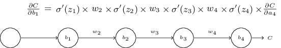
The structure of the expression is as follows: for each neuron in the network there is a multiplication term σ ′ (z _j ), for each weight there is w _j , and there is also the last term, ∂C / ∂a ₄ , corresponding to the cost function. Notice that I placed the corresponding members above the corresponding parts of the network. Therefore, the network itself is a mnemonic rule for expression.



You can take this expression on faith and skip its discussion right to the place where it is explained how it relates to the problem of the fading gradient. There is nothing wrong with this, as this expression is a special case from our discussion of backpropagation. However, it is easy to explain his fidelity, so it will be quite interesting (and perhaps instructive) for you to study this explanation.



Imagine that we made a small change in Δb ₁ to the offset b ₁ . This will send a series of cascading changes across the rest of the network. First, this will cause the output of the first hidden neuron Δa ₁ to change. This, in turn, force Δz ₂ to change in the weighted input to the second hidden neuron. Then there will be a change in Δa ₂ in the output of the second hidden neuron. And so on, up to a change in ΔC in the output value. It turns out that:

$$

$$\ frac {\ partial C} {\ partial b_1} \ approx \ frac {\ Delta C} {\ Delta b_1} \ tag {114}$$

This suggests that we can derive an expression for the gradient ∂C / ∂b ₁ , carefully monitoring the influence of each step in this cascade.



To do this, let us think how Δb ₁ causes the output a _{1 of the} first hidden neuron to change. We have a ₁ = σ (z ₁ ) = σ (w ₁ a ₀ + b ₁ ), therefore

$$

$$\ Delta a_1 \ approx \ frac {\ partial \ sigma (w_1 a_0 + b_1)} {\ partial b_1} \ Delta b_1 \ tag {115}$$

$$

$$= \ sigma '(z_1) \ Delta b_1 \ tag {116}$$

The term σ ′ (z ₁ ) should look familiar: this is the first term in our expression for the gradient ∂C / ∂b ₁ . Intuitively, it turns the change in the offset Δb ₁ into the change Δa _{1 of the} output activation. The change in Δa ₁ in turn causes a change in the weighted input z ₂ = w ₂ a ₁ + b _{2 of the} second hidden neuron:

$$

$$\ Delta z_2 \ approx \ frac {\ partial z_2} {\ partial a_1} \ Delta a_1 \ tag {117}$$

$$

$$= w_2 \ Delta a_1 \ tag {118}$$

Combining the expressions for Δz ₂ and Δa ₁ , we see how the change in the displacement b ₁ propagates along the network and affects z ₂ :

$$

$$\ Delta z_2 \ approx \ sigma '(z_1) w_2 \ Delta b_1 \ tag {119}$$

And this should also be familiar: these are the first two terms in our stated expression for the gradient ∂C / ∂b ₁ .



This can be continued further by monitoring how changes are propagated throughout the rest of the network. On each neuron, we select the term σ (z _j ), and through each weight we select the term w _j . The result is an expression relating the final change ΔC of the cost function with the initial change Δb _{1 of the} bias:

$$

$$\ Delta C \ approx \ sigma '(z_1) w_2 \ sigma' (z_2) \ ldots \ sigma '(z_4) \ frac {\ partial C} {\ partial a_4} \ Delta b_1 \ tag {120}$$

Dividing it by Δb ₁ , we really get the desired expression for the gradient:

$$

$$\ frac {\ partial C} {\ partial b_1} = \ sigma '(z_1) w_2 \ sigma' (z_2) \ ldots \ sigma '(z_4) \ frac {\ partial C} {\ partial a_4} \ tag { 121}$$

Why is there a fading gradient problem?

To understand why the disappearing gradient problem arises, let's write in detail our entire expression for the gradient:

$$

$$\ frac {\ partial C} {\ partial b_1} = \ sigma '(z_1) \ w_2 \ sigma' (z_2) \ w_3 \ sigma '(z_3) \, w_4 \ sigma' (z_4) \ \ frac {\ partial C} {\ partial a_4} \ tag {122}$$

In addition to the last term, this expression is the product of terms of the form w _j σ ′ (z _j ). To understand how each of them behaves, we look at the graph of the function σ:







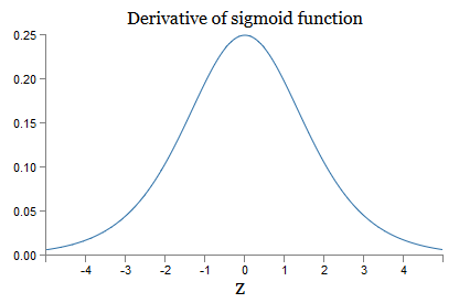
The graph reaches a maximum at the point σ ′ (0) = 1/4. If we use the standard approach to initializing the network weights, then we select the weights using the Gaussian distribution, that is, the root mean square zero and standard deviation 1. Therefore, usually the weights will satisfy the inequality | w _j | <1. Comparing all these observations, we see that the terms w _j σ ′ (z _j ) will usually satisfy the inequality | w _j σ ′ (z _j ) | <1/4. And if we take the product of the set of such terms, then it will decrease exponentially: the more members, the smaller the product. It starts to seem like a possible solution to the problem of the disappearing gradient.



To write this more accurately, we compare the expression for ∂C / ∂b ₁ with the expression of the gradient with respect to the next offset, for example, ∂C / ∂b ₃ . Of course, we did not write down a detailed expression for ∂C / ∂b ₃ , but it follows the same laws as described above for ∂C / ∂b ₁ . And here is a comparison of two expressions:







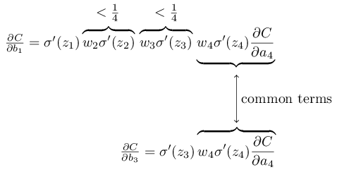
They have several common members. However, the gradient ∂C / ∂b ₁ includes two additional terms, each of which has the form w _j σ ′ (z _j ). As we have seen, such terms usually do not exceed 1/4. Therefore, the gradient ∂C / ∂b ₁ will usually be 16 (or more) times smaller than ∂C / ∂b ₃ . And this is the main cause of the disappearing gradient problem.



Of course, this is not accurate, but informal proof of the problem. There are several caveats. In particular, one may be interested in whether weights w _j will increase during training. If this happens, the terms w _j σ ′ (z _j ) in the product will no longer satisfy the inequality | w _j σ ′ (z _j ) | <1/4. And if they turn out to be large enough, more than 1, then we will no longer have the problem of a fading gradient. Instead, the gradient will grow exponentially as you move back through the layers. And instead of the disappearing gradient problem, we get the problem of explosive gradient growth.

The problem of explosive gradient growth

Let's look at a specific example of an explosive gradient. The example will be somewhat artificial: I will adjust the network parameters so as to guarantee the occurrence of explosive growth. But although the example is artificial, its plus is that it clearly demonstrates that the explosive growth of the gradient is not a hypothetical possibility, but it can really happen.



For explosive gradient growth, you need to take two steps. First, we choose large weights in the entire network, for example, w1 = w2 = w3 = w4 = 100. Then we choose such shifts so that the terms σ ′ (z _j ) are not too small. And this is quite easy to do: we only need to select such displacements so that the weighted input of each neuron is zj = 0 (and then σ ′ (z _j ) = 1/4). Therefore, for example, we need z ₁ = w ₁ a ₀ + b ₁ = 0. This can be achieved by assigning b ₁ = −100 ∗ a ₀ . The same idea can be used to select other offsets. As a result, we will see that all terms w _j σ ′ (z _j ) turn out to be equal to 100 ∗ 14 = 25. And then we get an explosive gradient growth.



Unstable gradient problem



The fundamental problem is not the disappearing gradient problem or the explosive growth of the gradient. It is that the gradient in the first layers is the product of members from all other layers. And when there are many layers, the situation essentially becomes unstable. And the only way that all layers will be able to learn at about the same speed is to choose such members of the work that will balance each other. And in the absence of some mechanism or reason for such balancing, it is unlikely that this will happen by chance.In short, the real problem is that NS suffer from the problem of an unstable gradient. And in the end, if we use standard gradient-based learning techniques, different layers of the network will learn at terribly different speeds.

Exercise

• , |σ′(z)|<1/4. , , . ?

We saw that the gradient can disappear or grow explosively in the first layers of a deep network. In fact, when using sigmoid neurons, the gradient will usually disappear. To understand why, again consider the expression | wσ ′ (z) |. To avoid the disappearing gradient problem, we need | wσ ′ (z) | ≥1. You may decide that this is easy to achieve with very large values ​​of w. However, in reality it is not so simple. The reason is that the term σ ′ (z) also depends on w: σ ′ (z) = σ ′ (wa + b), where a is the input activation. And if we make w large, we need to try not to make σ ′ (wa + b) small in parallel. And this turns out to be a serious limitation. The reason is that when we make w big, we make wa + b very big. If you look at the graph of σ ′, it can be seen that this leads us to the “wings” of the function σ ′,where it takes on very small values. And the only way to avoid this is to keep incoming activation in a fairly narrow range of values. Sometimes this happens by accident. But more often this does not happen. Therefore, in the general case, we have the problem of a vanishing gradient.

Tasks

• |wσ′(wa+b)|. , |wσ′(wa+b)|≥1. , , |w|≥4.
• , |w|≥4, , |wσ′(wa+b)|≥1.
• , , ,
  
  
  
  
  

  $$

  $$\frac{2}{|w|} \ln\left( \frac{|w|(1+\sqrt{1-4/|w|})}{2}-1\right) \tag{123}$$
  
  
  
  
  
• , |w|≈6.9, ≈0,45. , , , .
• . x, w ₁ , b w ₂ . , , , w ₂ σ(w ₁ x+b)≈x for x∈[0,1]. , , ( ). : x=1/2+Δ, , w ₁ , w ₁ Δ .

We studied toy networks with just one neuron in each hidden layer. What about more complex deep networks that have many neurons in each hidden layer?







In fact, much the same thing happens in such networks. Earlier in the chapter on back propagation, we saw that the gradient in layer #l of a network with L layers is specified as:

$$

$$\delta^l = \Sigma'(z^l) (w^{l+1})^T \Sigma'(z^{l+1}) (w^{l+2})^T \ldots \Sigma'(z^L) \nabla_a C \tag{124}$$

Here Σ ′ (z ^l ) is the diagonal matrix, whose elements are the values ​​of σ ′ (z) for the weighted inputs of layer No. l. w ^l are the weight matrices for different layers. And ∇ _a C is the vector of partial derivatives of C with respect to output activations.



This expression is much more complicated than the case with one neuron. And yet, if you look closely, its essence will be very similar, with a bunch of pairs of the form (w ^j ) ^T Σ ′ (z ^j ). Moreover, the matrices Σ ′ (z ^j ) diagonally have small values, not more than 1/4. If the weight matrices w ^j are not too large, each additional term (w ^j ) ^T Σ ′ (z ^l) tends to reduce the gradient vector, which leads to a disappearing gradient. In the general case, a larger number of multiplication terms leads to an unstable gradient, as in our previous example. In practice, empirically usually in sigmoid networks, gradients in the first layers disappear exponentially quickly. As a result, learning in these layers slows down. And the slowdown is not an accident or inconvenience: it is a fundamental consequence of our chosen approach to learning.

Other Barriers to Deep Learning

In this chapter, I focused on fading gradients - and more generally the case of unstable gradients - as an obstacle to deep learning. In fact, unstable gradients are just one obstacle to the development of civil defense, albeit an important and fundamental one. A significant part of current research is trying to better understand the problems that may arise in teaching GO. I will not describe all these works in detail, but I want to briefly mention a couple of works to give you an idea of ​​some questions asked by people.



As a first example in the work of 2010evidence was found that the use of sigmoid activation functions can lead to problems with learning NS. In particular, evidence was found that the use of a sigmoid will lead to the fact that the activations of the last hidden layer during training will be saturated in region 0, which will seriously slow down learning. Several alternative activation functions have been proposed that do not suffer so much from the saturation problem (see also another discussion paper ).



As a first example, in 2013, the effect of the random initialization of weights and the pulse graph in a stochastic gradient descent based on a pulse was studied on the GO. In both cases, a good choice significantly influenced the ability to train STS.



These examples suggest that the question “Why is the STS so difficult to train?” Is very complex. In this chapter, we focused on the instabilities associated with the gradient training of GNS. The results of the two previous paragraphs indicate that the choice of the activation function, the method of initializing the weights, and even the details of the implementation of training based on gradient descent also play a role. And, of course, the choice of network architecture and other hyperparameters will be important. Therefore, many factors can play a role in the difficulty of learning deep networks, and the issue of understanding these factors is the subject of ongoing research. But all this seems rather gloomy and inspires pessimism. However, there is good news - in the next chapter we will wrap everything in our favor, and we will develop several approaches in GO,which to some extent will be able to overcome or circumvent all these problems.