Reception of superlong radio waves at home
Ultra-long radio waves are a whole world filled with a multitude of signals — spherics and whistles generated by lightning, perhaps thousands of kilometers from the receiving point, the usual “points” and “dash” of Morzian, accurate time and digital data transmission signals:
Ultra Long Waves (ADD) (the term “ultra long waves” (UDV) was previously used)) - signals with a frequency of less than 30 kHz (according to the national classification). Abbreviations VLF ( very low frequenc y) and ELF ( extremely low frequency ) are often used abroad for this band, and the specific frequency bands for these bands differ in different sources.
The threshold of entry into this world is quite low - an antenna, an amplifier and a laptop with the appropriate software is required. Next, I will talk about my simple tackle for admission to ADD.
Antenna
To receive signals in the range of units - tens of kilohertz, I use a square-shaped antenna with a side length of 26 cm, wound with 50 turns of enameled copper wire with a radius of 0.1 mm and a winding resistance of 45 Ohms):
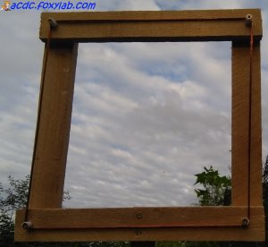
The directional pattern of the frame antenna in the horizontal plane (when the plane of the coils is arranged vertically) has the form of "eight":

If the plane of the frame is parallel to the direction of the radio station (the frame is “sideways”), then the level of the signal received by the framework antenna is maximum. If the plane of the frame is perpendicular to the direction of the radio station, the level of the received signal is minimal. This allows you to apply to determine the direction of the transmitter amplitude method with direction finding the minimum (more accurate than the maximum). The minimum of the received signal occurs in the direction perpendicular to the plane of the turns of the frame. Antenna with direction finding rotates to the position of zero reception.
Amplifier
To amplify the signal from the antenna, I use a two-stage amplifier (common emitter circuit) on bipolar transistors. Here is the model of this amplifier in LTspice :

I will not publish a photo of the amplifier in order not to cause anyone any moral suffering (it is assembled by my favorite method of gluing parts onto cardboard :-)).
The antenna is connected to the input of the amplifier with a coaxial cable to reduce noise.
Laptop / Netbook
The output of the amplifier is connected to the audio input (microphone or line) of a laptop or netbook. I use to digitize the input signal mode with a sampling frequency of 96 kHz 16 bit.
Software
To monitor the broadcast in real time, I use the Spectrum Lab program (you can download it here ) of version V2.90 b14 of the German radio amateur Wolfgang Büscher with the callsign DL4YHF :

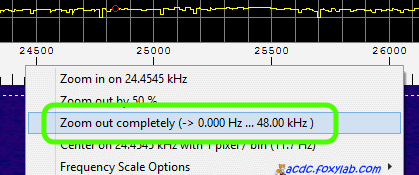
During the initial setup, I set the digitization frequency to 96 kHz:

and expanded the displayed frequency window for the whole range from 0 to 48 = 96/2 kHz:
An important role in setting up is the size of the Fourier transform window:

The window width affects the frequency and time resolution of the signal — as the window width increases, the frequency resolution increases, but the time resolution decreases and the computational cost of performing a fast Fourier transform increases.
The figure below shows the spectrograms of the signal with a window width of 1024 and 8192 reference:
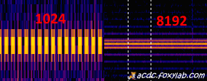
As can be seen, with a window width of 1024 counts, the pulse boundaries are clearly distinguishable, but the frequency of the pulses is blurred. With a window width of 8192 readings, the center frequency and the two extreme frequencies (upper and lower) are clearly traced, but the limits of the pulses are completely indistinguishable.
I also dabbled in MATLAB, trying to create an analyzer for weak signals:
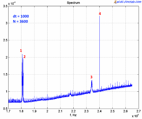
(GitHub - https://github.com/Dreamy16101976/VLF_MATLAB ).
Examples of signals received by me
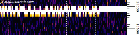
Frequency 25 kHz (call station radio RJH69)
Call Sign:

Time signals:

1 - 1/10 s, 2 - 1 s, 3 - 10 s, 4 - 60 s
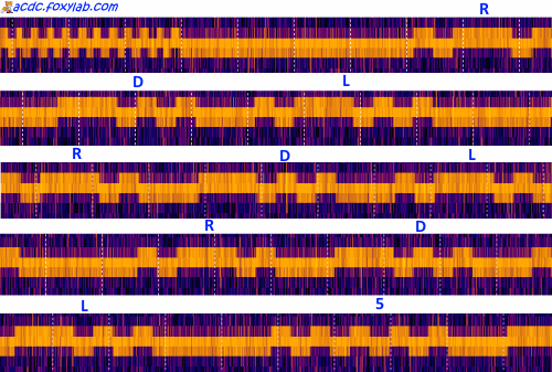
Frequency 18.1 kHz (callsign of a radio station RDL)
Types of signals:

1 - Unmodulated Carrier
2 - Sync signal (period duration about 60 ms)
3 - Sync signal (period duration about 40 ms)
4 - Digital data
5 - Morse code (the duration of one element is 1/15 s, i.e. the transfer rate is 18 wpm)
Call sign and radiogram beginning:
Interference
When add-on is extremely desirable to use a laptop battery power to reduce noise:
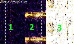
1 - laptop powered by battery
2 - powering the laptop from the battery, but the power supply is plugged in;
3 - mains powered laptop
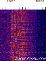
Very noticeable interference from the operation of the electronic ballast of compact fluorescent lamps at a frequency of about 40 kHz:

Such cases :-) Naturally, I covered only a small part of the world of ADD.
UPD Added video illustration to the article - https://youtu.be/cN-cLu3QIJk
Ultra Long Waves (ADD) (the term “ultra long waves” (UDV) was previously used)) - signals with a frequency of less than 30 kHz (according to the national classification). Abbreviations VLF ( very low frequenc y) and ELF ( extremely low frequency ) are often used abroad for this band, and the specific frequency bands for these bands differ in different sources.
Little history
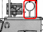
The first powerful ADL transmitter was commissioned in 1943 in Germany, and the “users” were reckless (it was unlikely that there was another branch of the war with such a percentage level of losses) from the Kriegsmarine submarine fleet. This is what the ADD antenna on the roof of the U-Boot cabin looked like:
The threshold of entry into this world is quite low - an antenna, an amplifier and a laptop with the appropriate software is required. Next, I will talk about my simple tackle for admission to ADD.
Antenna
To receive signals in the range of units - tens of kilohertz, I use a square-shaped antenna with a side length of 26 cm, wound with 50 turns of enameled copper wire with a radius of 0.1 mm and a winding resistance of 45 Ohms):
The directional pattern of the frame antenna in the horizontal plane (when the plane of the coils is arranged vertically) has the form of "eight":
If the plane of the frame is parallel to the direction of the radio station (the frame is “sideways”), then the level of the signal received by the framework antenna is maximum. If the plane of the frame is perpendicular to the direction of the radio station, the level of the received signal is minimal. This allows you to apply to determine the direction of the transmitter amplitude method with direction finding the minimum (more accurate than the maximum). The minimum of the received signal occurs in the direction perpendicular to the plane of the turns of the frame. Antenna with direction finding rotates to the position of zero reception.
Amplifier
To amplify the signal from the antenna, I use a two-stage amplifier (common emitter circuit) on bipolar transistors. Here is the model of this amplifier in LTspice :
I will not publish a photo of the amplifier in order not to cause anyone any moral suffering (it is assembled by my favorite method of gluing parts onto cardboard :-)).
The antenna is connected to the input of the amplifier with a coaxial cable to reduce noise.
Laptop / Netbook
The output of the amplifier is connected to the audio input (microphone or line) of a laptop or netbook. I use to digitize the input signal mode with a sampling frequency of 96 kHz 16 bit.
Software
To monitor the broadcast in real time, I use the Spectrum Lab program (you can download it here ) of version V2.90 b14 of the German radio amateur Wolfgang Büscher with the callsign DL4YHF :
During the initial setup, I set the digitization frequency to 96 kHz:
and expanded the displayed frequency window for the whole range from 0 to 48 = 96/2 kHz:
An important role in setting up is the size of the Fourier transform window:
The window width affects the frequency and time resolution of the signal — as the window width increases, the frequency resolution increases, but the time resolution decreases and the computational cost of performing a fast Fourier transform increases.
The figure below shows the spectrograms of the signal with a window width of 1024 and 8192 reference:
As can be seen, with a window width of 1024 counts, the pulse boundaries are clearly distinguishable, but the frequency of the pulses is blurred. With a window width of 8192 readings, the center frequency and the two extreme frequencies (upper and lower) are clearly traced, but the limits of the pulses are completely indistinguishable.
I also dabbled in MATLAB, trying to create an analyzer for weak signals:
(GitHub - https://github.com/Dreamy16101976/VLF_MATLAB ).
Examples of signals received by me
Frequency 25 kHz (call station radio RJH69)
Call Sign:
Time signals:
1 - 1/10 s, 2 - 1 s, 3 - 10 s, 4 - 60 s
Frequency 18.1 kHz (callsign of a radio station RDL)
Types of signals:
1 - Unmodulated Carrier
2 - Sync signal (period duration about 60 ms)
3 - Sync signal (period duration about 40 ms)
4 - Digital data
5 - Morse code (the duration of one element is 1/15 s, i.e. the transfer rate is 18 wpm)
Call sign and radiogram beginning:
Interference
When add-on is extremely desirable to use a laptop battery power to reduce noise:
1 - laptop powered by battery
2 - powering the laptop from the battery, but the power supply is plugged in;
3 - mains powered laptop
Very noticeable interference from the operation of the electronic ballast of compact fluorescent lamps at a frequency of about 40 kHz:
Such cases :-) Naturally, I covered only a small part of the world of ADD.
UPD Added video illustration to the article - https://youtu.be/cN-cLu3QIJk
All Articles