Wireless power transmission through magnetically coupled inductive coils

Introduction

I think that many of the readers have seen at least one video on popular video services, where electricity is transmitted through empty space using inductive coils.

In this article, we want to address the fundamentals of the process of wireless energy transmission using a magnetic field. Starting with consideration of the simplest inductive coil, and calculating its inductance, we will gradually move on to the theory of electrical circuits, in the framework of which the method of transmitting maximum power will be shown and justified under other equal conditions. So, let's begin.

Magnetic field of a single coil with current

Consider the magnetic field of a single coil with a current. Find the magnetic field of the coil at any point in space. Why is such a review necessary? Because in almost all books, at least in those that the author of the article was able to find, the solution to this problem is limited to finding only one component of the magnetic field and only along the axis of the coil -

B_{z} (z)

$B_z (z)$ , while we will find the law for the magnetic field in the whole space.

Magnetic field of a single coil with current

Illustration to the law of Bio-Savard-Laplace

To find the magnetic field, we use the law of Bio-Savart-Laplace (see Wikipedia - the Law of Bio-Savard-Laplace ). The figure shows that the center of the coordinate system

O

$O$ coincides with the center of the coil. The contour of the circle of the coil is indicated as

C

$C$ , and the radius of the circle - as

a

$a$ . During the coil current flows

I

$I$ .

v e c r

$\ vec {r}$ - is a variable-radius-vector from the origin to an arbitrary point of the coil.

v e c r_{0}

$\ vec {r} _0$ Is the radius vector to the observation point. We also need a polar angle.

v a r p h i

$\ varphi$ - the angle between the radius vector

v e c r

$\ vec {r}$ and axis

O X

$OX$ . The distance from the axis of the turn to the observation point is denoted by

r h o

$\ rho$ . And finally

m a t h r m d v e c r

$\ mathrm {d} \ vec {r}$ - elementary increment of the radius-vector

v e c r

$\ vec {r}$ .

According to the law of Bio-Savard-Laplace, the circuit element with current

m a t h r m d v e c r

$\ mathrm {d} \ vec {r}$ creates an elementary contribution to the magnetic field, which is given by the formula

m a t h r m d v e c B (v e c r_{0}) = f r a c m u_{0} I 4 p i c d o t f r a c [m a t h r m d v e c r t i m e s (v e c r_{0} - v e c r)] | v e c r_{0} - v e c r |^{3}

$\ mathrm {d} \ vec {B} (\ vec {r} _0) = \ frac {\ mu_0 I} {4 \ pi} \ cdot \ frac {[\, \ mathrm {d} \ vec {r} \ times (\ vec {r} _0- \ vec {r})]} {| \ vec {r} _0- \ vec {r} | ^ 3}$

Now we’ll dwell on the variables and expressions included in the formula. Given the axial symmetry of the problem, we can write

v e c r_{0} = (r h o c o s v a r p h i, r h o s i n v a r p h i, z) o v e r s e t v a r p h i = 0 r i g h t a r r o w (r h o, 0, z)

$\ vec {r} _0 = (\ rho \ cos {\ varphi}, \ rho \ sin {\ varphi}, z) \ overset {\ varphi = 0} {\ rightarrow} (\ rho, 0, z)$

v e c r = (a c o s v a r p h i, a s i n v a r p h i, 0)

$\ vec {r} = (a \ cos {\ varphi}, a \ sin {\ varphi}, 0)$

m a t h r m d v e c r = (- a s i n v a r p h i, a c o s v a r p h i, 0) m a t h r m d v a r p h i

$\ mathrm {d} \ vec {r} = (-a \ sin {\ varphi}, a \ cos {\ varphi}, 0) \, \ mathrm {d} \ varphi$

v e c r_{0} - v e c r = (r h o - a c o s v a r p h i, - a s i n v a r p h i, z)

$\ vec {r} _0- \ vec {r} = (\ rho -a \ cos {\ varphi}, -a \ sin {\ varphi}, z)$

[\ mathrm {d} \ vec {r} \ times (\ vec {r} _0- \ vec {r})] = \ begin {vmatrix} \ vec {e} _x & \ vec {e} _y & \ vec { e} _z \\ -a \ sin {\ varphi} \, \ mathrm {d} \ varphi & a \ cos {\ varphi} \, \ mathrm {d} \ varphi & 0 \\ \ rho -a \ cos {\ varphi } & -a \ sin {\ varphi} & z \ end {vmatrix} = (az \ cos {\ varphi}, az \ sin {\ varphi}, a ^ 2 -a \ rho \ cos {\ varphi}) \ , \ mathrm {d} \ varphi

$[\ mathrm {d} \ vec {r} \ times (\ vec {r} _0- \ vec {r})] = \ begin {vmatrix} \ vec {e} _x & \ vec {e} _y & \ vec { e} _z \\ -a \ sin {\ varphi} \, \ mathrm {d} \ varphi & a \ cos {\ varphi} \, \ mathrm {d} \ varphi & 0 \\ \ rho -a \ cos {\ varphi } & -a \ sin {\ varphi} & z \ end {vmatrix} = (az \ cos {\ varphi}, az \ sin {\ varphi}, a ^ 2 -a \ rho \ cos {\ varphi}) \ , \ mathrm {d} \ varphi$

| v e c r_{0} - v e c r |^{3} = l e f t (r h o^{2} + a^{2} + z^{2} - 2 r h o a c o s v a r p h i r i g h t)^{f r a c 32}

$| \ vec {r} _0- \ vec {r} | ^ 3 = \ left (\ rho ^ 2 + a ^ 2 + z ^ 2 -2 \ rho a \ cos {\ varphi} \ right) ^ {\ frac {3} {2}}$

In order to find the resultant magnetic field, it is necessary to integrate over the whole loop contour, i.e.

v e c B (v e c r_{0}) = i n t_{C} m a t h r m d v e c B (v e c r_{0})

$\ vec {B} (\ vec {r} _0) = \ int_C {\, \ mathrm {d} \ vec {B} (\ vec {r} _0)}$

After the substitution of all expressions and some identical transformations, we obtain expressions for the axial and radial components of the magnetic field, respectively

B_{z} (r h o, z) = f r a c m u_{0} I 4 p i i n t_{0}^{2 p i} f r a c l e f t (a^{2} - r h o a c o s v a r p h i r i g h t) m a t h r m d v a r p h i l e f t (r h o^{2} + a^{2} + z^{2} - 2 r h o a c o s v a r p h i r i g h t)^{f r a c 32}

$B_z (\ rho, z) = \ frac {\ mu_0 I} {4 \ pi} \ int_0 ^ {2 \ pi} {\ frac {\ left (a ^ 2 - \ rho a \ cos {\ varphi} \ right) \, \ mathrm {d} \ varphi} {\ left (\ rho ^ 2 + a ^ 2 + z ^ 2 -2 \ rho a \ cos {\ varphi} \ right) ^ {\ frac {3} { 2}}}}$

B_{r} (r h o, z) = f r a c m u_{0} I 4 p i i n t_{0}^{2 p i} f r a c a z m a t h r m d v a r p h i l e f t (r h o^{2} + a^{2} + z^{2} - 2 r h o a c o s v a r p h i r i g h t)^{f r a c 32}

$B_r (\ rho, z) = \ frac {\ mu_0 I} {4 \ pi} \ int_0 ^ {2 \ pi} {\ frac {a \, z \, \, \ mathrm {d} \ varphi} { \ left (\ rho ^ 2 + a ^ 2 + z ^ 2 -2 \ rho a \ cos {\ varphi} \ right) ^ {\ frac {3} {2}}}}$

To find the absolute value of the magnetic field, it is necessary to sum up the components according to the Pythagorean theorem

B = s q r t B_{r}^{2} + B_{z}^{2}

$B = \ sqrt {B_r ^ 2 + B_z ^ 2}$ .

Let us demonstrate the solution obtained using the example of a radius coil

a = 0.1

$a = 0.1$ (m) and

I = 1

$I = 1$ (BUT).

Axial magnetic field amplitude

The amplitude of the axial component of the magnetic field

The amplitude of the radial magnetic field

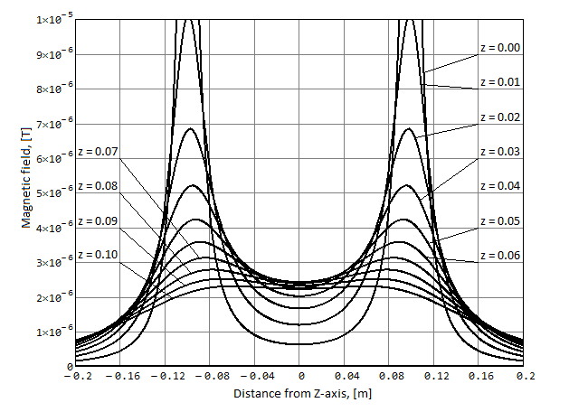
The amplitude of the radial component of the magnetic field

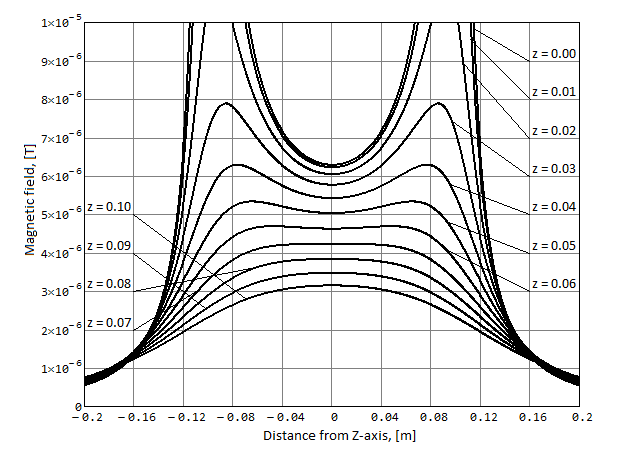
Absolute magnetic field amplitude

Note that for a coil of arbitrary shape, at large distances

z g g a

$z \ gg a$ i.e. much larger than the characteristic size of the coil, the behavior of the magnetic field will tend to the solution found.

Hint...

For such calculations and graphing is convenient to use MathCad 15

Inductor. Magnetically coupled coils

Now that we know the solution for the magnetic field of a single turn, we can find the inductance of the coil, consisting of

n

$n$ turns. By definition, inductance is the coefficient of proportionality between the current in a coil and the magnetic flux through the cross section area. Here we use the ideal coil model, which is dimensionless in the direction of its axis of symmetry. Of course, in practice this does not happen. However, as approximations, the formulas obtained will be good enough. Although coils are considered dimensionless along

O Z

$OZ$ , you must specify a non-zero radius of the wire cross section. Denote it

d e l t a

$\ delta$ and example equal

d e l t a = $ 0.

$\ delta = $ 0.$ (mm) Otherwise, when integrating the magnetic flux, the integrand will turn to infinity.

inductively coupled coils

Inductively connected coils

The figure shows two magnetically coupled coils. Let the first coil have a radius

a_{1}

$a_1$ and contains

n_{1}

$n_1$ turns, and the second -

a_{2}

$a_2$ and

n_{2}

$n_2$ respectively. Then, in order to find the own inductances, it is necessary to calculate the magnetic flux of each coil through its own section.

\ Phi = \ iint_S {\ vec {B} \ cdot \ vec {\, \ mathrm {d} S}} = \ int_0 ^ {2 \ pi} {\ int_0 ^ {a- \ delta} {B_z (\ rho, z) \ rho \, \ mathrm {d} \ rho \, \ mathrm {d} \ varphi} = 2 \ pi \ int_0 ^ {a- \ delta} {B_z (\ rho, z) \ rho \ , \ mathrm {d} \ rho}

$\ Phi = \ iint_S {\ vec {B} \ cdot \ vec {\, \ mathrm {d} S}} = \ int_0 ^ {2 \ pi} {\ int_0 ^ {a- \ delta} {B_z (\ rho, z) \ rho \, \ mathrm {d} \ rho \, \ mathrm {d} \ varphi} = 2 \ pi \ int_0 ^ {a- \ delta} {B_z (\ rho, z) \ rho \ , \ mathrm {d} \ rho}$

Since there are many turns in the coil, we find the quantity called the flux linkage, by multiplying twice the number of turns

P s i = f r a c 12 n^{2} m u_{0} I i n t_{0}^{a - d e l t a} i n t_{0}^{2 p i} f r a c l e f t (a^{2} - r h o a c o s v a r p h i r i g h t) m a t h r m d v a r p h i l e f t (r h o^{2} + a^{2} + z^{2} - 2 r h o a c o s v a r p h i r i g h t)^{f r a c 32} r h o m a t h r m d r h o

$\ Psi = \ frac {1} {2} n ^ 2 \ mu_0 I \ int_0 ^ {a- \ delta} {\ int_0 ^ {2 \ pi} {\ frac {\ left (a ^ 2 - \ rho a \ cos {\ varphi} \ right) \, \ mathrm {d} \ varphi} {\ left (\ rho ^ 2 + a ^ 2 + z ^ 2 -2 \ rho a \ cos {\ varphi} \ right) ^ {\ frac {3} {2}}}} \ rho \, \ mathrm {d} \ rho}$

By definition, inductance is a coefficient of proportionality

L

$L$ in the formula

P s i = L I

$\ Psi = LI$ . Thus, we obtain the own inductances of the coils

L_{1} = f r a c 12 n_{1}^{2} m u_{0} i n t_{0}^{a_{1} - d e l t a} i n t_{0}^{2 p i} f r a c l e f t (a_{1}^{2} - r h o a_{1} c o s v a r p h i r i g h t) m a t h r m d v a r p h i l e f t (r h o^{2} + a_{1}^{2} - 2 r h o a_{1} c o s v a r p h i r i g h t)^{f r a c 32} r h o m a t h r m d r h o

$L_1 = \ frac {1} {2} n_1 ^ 2 \ mu_0 \ int_0 ^ {a_1- \ delta} {\ int_0 ^ {2 \ pi} {\ frac {\ left (a_1 ^ 2 - \ rho a_1 \ cos {\ varphi} \ right) \, \ mathrm {d} \ varphi} {\ left (\ rho ^ 2 + a_1 ^ 2 -2 \ rho a_1 \ cos {\ varphi} \ right) ^ {\ frac {3} {2}}}} \ rho \, \ mathrm {d} \ rho}$

L_{2} = f r a c 12 n_{2}^{2} m u_{0} i n t_{0}^{a_{2} - d e l t a} i n t_{0}^{2 p i} f r a c l e f t (a_{2}^{2} - r h o a_{2} c o s v a r p h i r i g h t) m a t h r m d v a r p h i l e f t (r h o^{2} + a_{2}^{2} - 2 r h o a_{2} c o s v a r p h i r i g h t)^{f r a c 32} r h o m a t h r m d r h o

$L_2 = \ frac {1} {2} n_2 ^ 2 \ mu_0 \ int_0 ^ {a_2- \ delta} {\ int_0 ^ {2 \ pi} {\ frac {\ left (a_2 ^ 2 - \ rho a_2 \ cos {\ varphi} \ right) \, \ mathrm {d} \ varphi} {\ left (\ rho ^ 2 + a_2 ^ 2 -2 \ rho a_2 \ cos {\ varphi} \ right) ^ {\ frac {3} {2}}}} \ rho \, \ mathrm {d} \ rho}$

Let the centers of the coils be separated by distance

d

$d$ , lie on the same axis, and their plane of turns is oriented parallel. To find the mutual inductance, it is necessary to calculate the flux linkage formed by one coil through the cross section of another, i.e.

P s i_{12} = f r a c 12 n_{1} n_{2} m u_{0} I i n t_{0}^{a_{2} - d e l t a} i n t_{0}^{2 p i} f r a c l e f t (a_{1}^{2} - r h o a_{1} c o s v a r p h i r i g h t) m a t h r m d v a r p h i l e f t (r h o^{2} + a_{1}^{2} + z^{2} - 2 r h o a_{1} c o s v a r p h i r i g h t)^{f r a c 32} r h o m a t h r m d r h o

$\ Psi_ {12} = \ frac {1} {2} n_1 n_2 \ mu_0 I \ int_0 ^ {a_2- \ delta} {\ int_0 ^ {2 \ pi} {\ frac {\ left (a_1 ^ 2 - \ rho a_1 \ cos {\ varphi} \ right) \, \ mathrm {d} \ varphi} {\ left (\ rho ^ 2 + a_1 ^ 2 + z ^ 2 -2 \ rho a_1 \ cos {\ varphi} \ right ) ^ {\ frac {3} {2}}}} \ rho \, \ mathrm {d} \ rho}$

Then the mutual inductance of the coils is given by

M_{12} = f r a c 12 n_{1} n_{2} m u_{0} i n t_{0}^{a_{2} - d e l t a} i n t_{0}^{2 p i} f r a c l e f t (a_{1}^{2} - r h o a_{1} c o s v a r p h i r i g h t) m a t h r m d v a r p h i l e f t (r h o^{2} + a_{1}^{2} + d^{2} - 2 r h o a_{1} c o s v a r p h i r i g h t)^{f r a c 32} r h o m a t h r m d r h o

$M_ {12} = \ frac {1} {2} n_1 n_2 \ mu_0 \ int_0 ^ {a_2- \ delta} {\ int_0 ^ {2 \ pi} {\ frac {\ left (a_1 ^ 2 - \ rho a_1 \ cos {\ varphi} \ right) \, \ mathrm {d} \ varphi} {\ left (\ rho ^ 2 + a_1 ^ 2 + d ^ 2 -2 \ rho a_1 \ cos {\ varphi} \ right) ^ {\ frac {3} {2}}}} \ rho \, \ mathrm {d} \ rho}$

As far as the author knows, such integrals can be taken only numerically.

Note that as a rule

P s i_{12} = P s i_{21}

$\ Psi_ {12} = \ Psi_ {21}$ and

M_{12} = M_{21} = M

$M_ {12} = M_ {21} = M$ . Coil coupling coefficient is called magnitude

k = f r a c M s q r t L_{1} L_{2}

$k = \ frac {M} {\ sqrt {L_1L_2}}$

We investigate the dependence of the coupling coefficient of the coils on the distance. To do this, consider two identical coils with a radius of turns

a_{1} = a_{2} = 0.1

$a_1 = a_2 = 0.1$ (m) and the number of turns

n_{1} = n_{2} = 100

$n_1 = n_2 = 100$ . In this case, the inductance of each of the coils will be

L_{1} = L_{2} = 8.775

$L_1 = L_2 = 8.775$ (mH).

Graph of the coupling coefficient of two identical coils on the distance between them

Coil coupling ratio of the distance between them

The schedule will not change if the number of turns in both coils is equally changed, or the radius of both coils is equally changed. The coupling coefficient is conveniently expressed as a percentage. From the graph it is seen that even with the distance between the coils of 1 (mm), the coupling coefficient is less than 100%. The coefficient drops to 10% at a distance of about 60 (mm), and to 1% at 250 (mm).

Wireless power transmission

So, we know inductance and coupling coefficient. Now let us use the theory of electrical circuits of alternating current to find the optimal parameters at which the transmitted power would be maximum. To understand this paragraph, the reader must be familiar with the concept of electrical impedance, as well as Kirchhoff's laws and Ohm's law. As is known from the theory of circuits, two inductively coupled coils form an air transformer. For the analysis of transformers convenient T-shaped equivalent circuit.

Air transformer and its equivalent circuit

The transmitting coil on the left will be called the "trasmitter", and the receiving coil on the right will be called the "receiver". Between coils coupling coefficient

k

$k$ . On the side of the receiver is the consumer represented by the load

z_{L}

$z_L$ . The load can generally be complex. Input voltage on the transmitter side

u_{1}

$u_1$ and input current -

i_{1}

$i_1$ . The voltage transmitted to the receiver -

u_{2}

$u_2$ and current transmitted

i_{2}

$i_2$ . The full impedance on the transmitter side is denoted as

z_{1}

$z_1$ , and the full impedance on the side of the receiver

z_{2}

$z_2$ .

It is assumed that a sinusoidal voltage is applied to the input of the circuit.

u_{1} = u_{1 m} s i n o m e g a t

$u_1 = u_ {1m} \ sin {\ omega t}$ .

Denote

R_{c o i l 1}, R_{c o i l 2}, L_{c o i l 1}, L_{c o i l 2}, M

$R_ {coil \, 1}, R_ {coil \, 2}, L_ {coil \, 1}, L_ {coil \, 2}, M$ - resistance and inductance of the coils (two own and one mutual), respectively. Then, according to transformer theory

z_{1} = R_{c o i l 1} + j o m e g a (L_{c o i l 1} - M)

$z_1 = R_ {coil \, 1} + j \ omega (L_ {coil \, 1} - M)$

z_{2} = R_{c o i l 2} + j o m e g a (L_{c o i l 2} - M) + R_{l o a d} + j X_{l o a d}

$z_2 = R_ {coil \, 2} + j \ omega (L_ {coil \, 2} - M) + R_ {load} + j X_ {load}$

On the other hand, according to our designations

z_{1} = r_{1} + j x_{1}

$z_1 = r_1 + j x_1$

z_{2} = r_{2} + j x_{2}

$z_2 = r_2 + j x_2$

Where

r_{1}, r_{2}

$r_1, r_2$ - total resistances on the side of the transmitter and receiver, respectively, and

x_{1}, x_{2}

$x_1, x_2$ - full reactive resistances.

Communication impedance is

z_{3} = j o m e g a M = j x_{3}

$z_3 = j \ omega M = j x_3$ .

Find the input current of the circuit

i_{1} = f r a c u_{1} z_{1} + z_{2} | | z_{3}

$i_1 = \ frac {u_1} {z_1 + z_2 || z_3}$

where is the sign

| |

$||$ denotes a parallel connection of resistances. Then the voltage transmitted to the receiver

u_{2} = u_{1} - i_{1} z_{1} = u_{1} l e f t (1 - f r a c z_{1} z_{1} + z_{2} | | z_{3} r i g h t)

$u_2 = u_1 - i_1 z_1 = u_1 \ left (1 - \ frac {z_1} {z_1 + z_2 || z_3} \ right)$

And induced current

i_{2} = f r a c u_{2} z_{2} = f r a c u_{1} z_{2} l e f t (1 - f r a c z_{1} z_{1} + z_{2} | | z_{3} r i g h t)

$i_2 = \ frac {u_2} {z_2} = \ frac {u_1} {z_2} \ left (1 - \ frac {z_1} {z_1 + z_2 || z_3} \ right)$

We can find the integrated power transmitted to the receiver

s_{2} = u_{2} i_{2}^{*} = p_{2} + j q_{2}

$s_2 = u_2 i_2 ^ * = p_2 + jq_2$

Thus, we have an expression for the complex power

s_{2} = | u_{1} |^{2} z_{2} l e f t | f r a c z_{3} z_{1} z_{2} + z_{1} z_{3} + z_{2} z_{3} r i g h t |^{2}

$s_2 = | u_1 | ^ 2 z_2 \ left | \ frac {z_3} {z_1z_2 + z_1z_3 + z_2z_3} \ right | ^ 2$

Expression for active power component

p_{2} = | u_{1} |^{2} r_{2} l e f t | f r a c z_{3} z_{1} z_{2} + z_{1} z_{3} + z_{2} z_{3} r i g h t |^{2}

$p_2 = | u_1 | ^ 2 r_2 \ left | \ frac {z_3} {z_1z_2 + z_1z_3 + z_2z_3} \ right | ^ 2$

Expression for reactive power components

q_{2} = | u_{1} |^{2} x_{2} l e f t | f r a c z_{3} z_{1} z_{2} + z_{1} z_{3} + z_{2} z_{3} r i g h t |^{2}

$q_2 = | u_1 | ^ 2 x_2 \ left | \ frac {z_3} {z_1z_2 + z_1z_3 + z_2z_3} \ right | ^ 2$

In most practical tasks, the maximum active power is required, therefore

p_{2} r i g h t a r r o w m a t h r m m a x R i g h t a r r o w l e f t | f r a c z_{3} z_{1} z_{2} + z_{1} z_{3} + z_{2} z_{3} r i g h t |^{2} r i g h t a r r o w m a t h r m m a x

$p_2 \ rightarrow \ mathrm {max} \ Rightarrow \ left | \ frac {z_3} {z_1z_2 + z_1z_3 + z_2z_3} \ right | ^ 2 \ rightarrow \ mathrm {max}$

Either that same

l e f t | z_{1} + z_{2} + f r a c z_{1} z_{2} z_{3} r i g h t |^{2} r i g h t a r r o w m a t h r m m i n

$\ left | z_1 + z_2 + \ frac {z_1z_2} {z_3} \ right | ^ 2 \ rightarrow \ mathrm {min}$

l e f t | r_{1} + j x_{1} + r_{2} + j x_{2} + f r a c (r_{1} + j x_{1}) (r_{2} + j x_{2}) j x_{3} r i g h t |^{2} r i g h t a r r o w m a t h r m m i n

$\ left | r_1 + jx_1 + r_2 + jx_2 + \ frac {(r_1 + jx_1) (r_2 + jx_2)} {jx_3} \ right | ^ 2 \ rightarrow \ mathrm {min}$

f r a c 1 x_{3}^{2} | (r_{1} x_{3} + r_{2} x_{3} + r_{1} x_{2} + r_{2} x_{1}) + j (x_{1} x_{3} + x_{2} x_{3} + x_{1} x_{2} - r_{1} r_{2}) |^{2} r i g h t a r r o w m a t h r m m i n

$\ frac {1} {x_3 ^ 2} | (r_1x_3 + r_2x_3 + r_1x_2 + r_2x_1) + j (x_1x_3 + x_2x_3 + x_1x_2 - r_1r_2) | ^ 2 \ rightarrow \ mathrm {min}$

For convenience, we introduce the function

f (x_{1}, x_{2}) = (r_{1} x_{3} + r_{2} x_{3} + r_{1} x_{2} + r_{2} x_{1}) + j (x_{1} x_{3} + x_{2} x_{3} + x_{1} x_{2} - r_{1} r_{2})

$f (x_1, x_2) = (r_1x_3 + r_2x_3 + r_1x_2 + r_2x_1) + j (x_1x_3 + x_2x_3 + x_1x_2 - r_1r_2)$

and examine it for extremes

| f (x_{1}, x_{2}) |^{2} r i g h t a r r o w m a t h r m m i n

$| f (x_1, x_2) | ^ 2 \ rightarrow \ mathrm {min}$

Where do we get a system of two equations

f r a c p a r t i a l | f |^{2} p a r t i a l x_{1} = 2 m a t h b b R e (f) r_{2} + 2 m a t h b b I m (f) (x_{2} + x_{3}) = 0

$\ frac {\ partial | f | ^ 2} {\ partial x_1} = 2 \ mathbb {Re} (f) r_2 + 2 \ mathbb {Im} (f) (x_2 + x_3) = 0$

f r a c p a r t i a l | f |^{2} p a r t i a l x_{2} = 2 m a t h b b R e (f) r_{1} + 2 m a t h b b I m (f) (x_{1} + x_{3}) = 0

$\ frac {\ partial | f | ^ 2} {\ partial x_2} = 2 \ mathbb {Re} (f) r_1 + 2 \ mathbb {Im} (f) (x_1 + x_3) = 0$

This system has five solutions, two of which are nonphysical, since they lead to imaginary values of quantities that are supposed to be valid. Three other physical solutions are given below, together with the corresponding power formulas.

Solution 1

x_{1} = - x_{3}, q u a d x_{2} = - x_{3}

$x_1 = -x_3, \ quad x_2 = -x_3$

Power

p_{2} = f r a c | u_{1} |^{2} x_{3}^{2} r_{2} l e f t (r_{1} r_{2} + x_{3}^{2} r i g h t)^{2}, q u a d q_{2} = - f r a c | u_{1} |^{2}, x_{3}^{3} l e f t (r_{1} r_{2} + x_{3}^{2} r i g h t)^{2}

$p_2 = \ frac {| u_1 | ^ 2 \, x_3 ^ 2 \, r_2} {\ left (r_1r_2 + x_3 ^ 2 \ right) ^ 2}, \ quad q_2 = - \ frac {| u_1 | ^ 2 \ , x_3 ^ 3} {\ left (r_1r_2 + x_3 ^ 2 \ right) ^ 2}$

Solution 2 and 3

x_{1} = f r a c 1 r_{2} l e f t (s q r t r_{1} r_{2} l e f t (x_{3}^{2} - r_{1} r_{2} r i g h t) - ​ ​ r_{2} x_{3} r i g h t), q u a d x_{2} = f r a c 1 r_{1} l e f t (s q r t r_{1} r_{2} l e f t (x_{3}^{2} - r_{1} r_{2} r i g h t) - ​ ​ r_{1} x_{3} r i g h t)

$x_1 = \ frac {1} {r_2} \ left (\ sqrt {r_1r_2 \ left (x_3 ^ 2-r_1r_2 \ right)} - r_2x_3 \ right), \ quad x_2 = \ frac {1} {r_1} \ left (\ sqrt {r_1r_2 \ left (x_3 ^ 2-r_1r_2 \ right)} - r_1x_3 \ right)$

x_{1} = - f r a c 1 r_{2} l e f t (s q r t r_{1} r_{2} l e f t (x_{3}^{2} - r_{1} r_{2} r i g h t) + r_{2} x_{3} r i g h t), q u a d x_{2} = - f r a c 1 r_{1} l e f t (s q r t r_{1} r_{2} l e f t (x_{3}^{2} - r_{1} r_{2} r i g h t) + r_{1} x_{3} r i g h t)

$x_1 = - \ frac {1} {r_2} \ left (\ sqrt {r_1r_2 \ left (x_3 ^ 2-r_1r_2 \ right)} + r_2x_3 \ right), \ quad x_2 = - \ frac {1} {r_1} \ left (\ sqrt {r_1r_2 \ left (x_3 ^ 2-r_1r_2 \ right)} + r_1x_3 \ right)$

Power for solutions 2 and 3

p_{2} = f r a c | u_{1} |^{2} 4 r_{1}, q u a d q_{2} = f r a c | u_{1} |^{2} x_{2} 4 r_{1} r_{2}

$p_2 = \ frac {| u_1 | ^ 2} {4 \, r_1}, \ quad q_2 = \ frac {| u_1 | ^ 2 \, x_2} {4 \, r_1 \, r_2}$

Solution 2 and 3 should be used when the coupling reactance is large enough.

x_{3}^{2} > r_{1} r_{2}

$x_3 ^ 2> r_1r_2$

When this is not the case, you need to use solution 1. Most often in real situations

x_{3}

$x_3$ will be small, so consider solution 1 in some detail.

Solution 1:

x_{1} = - x_{3}, q u a d x_{2} = - x_{3}

$x_1 = -x_3, \ quad x_2 = -x_3$ . And the corresponding active power is given by the formula

p_{2} = f r a c | u_{1} |^{2} x_{3}^{2} r_{2} l e f t (r_{1} r_{2} + x_{3}^{2} r i g h t)^{2}

$p_2 = \ frac {| u_1 | ^ 2 \, x_3 ^ 2 \, r_2} {\ left (r_1r_2 + x_3 ^ 2 \ right) ^ 2}$

It can be seen from the power formula that the power depends on the reactance of the connection

x_{3} = 2 p i f k s q r t L_{c o i l 1} L_{c o i l 2}

$x_3 = 2 \ pi \, f \, k \, \ sqrt {L_ {coil \, 1} L_ {coil \, 2}}$ and therefore from the transmission frequency

f

$f$ , and from the geometry of the relative position of the coils, which is taken into account by the coupling coefficient

k

$k$ .

As attentive readers noticed, addiction

p_{2} (x_{3})

$p_2 (x_3)$ - nonlinear. Function

p_{2} (x_{3})

$p_2 (x_3)$ reaches a maximum at

x_{3} = s q r t r_{1} r_{2}

$x_3 = \ sqrt {r_1r_2}$ .

The study of the power formula for extremes

Power formula research

$p_2 (x_3)$ on extremes

Maximum active power at

x_{3} = s q r t r_{1} r_{2}

$x_3 = \ sqrt {r_1r_2}$ equals

p_{2} = f r a c | u_{1} |^{2} 4 r_{1}

$p_2 = \ frac {| u_1 | ^ 2} {4 \, r_1}$

Thus, the above formula represents the absolute theoretical limit of the transmitted active power under any conditions. For reactive power transmitted to the receiver, we have

q_{2} = f r a c | u_{1} |^{2} s q r t r_{1} r_{2}

$q_2 = \ frac {| u_1 | ^ 2} {\ sqrt {r_1r_2}}$

Numerical simulation

You can demonstrate the work of the above theory by running the SPICE simulation of the model of our device from two coupled coils.

SPICE model of two inductively coupled coils

Simulation performed for coupling coefficient

k = 1

$k = 1$ %, which corresponds to 25 cm removal between the coils. The parameters of the coils are the same as in the previous paragraph, adopted for plotting

k

$k$ .

It turns out that the reactances of each of the coils must be compensated for by capacitors.

С_{1}

$_1$ and

C_{2}

$C_2$ . That is, adjust each of the circuits (transmitting and receiving) to resonance at a given frequency. If we assume that the load value is real, then the values of the containers can be found from the formulas

C_{1} = f r a c 1 o m e g a^{2} L_{1}, q u a d C_{2} = f r a c 1 o m e g a^{2} L_{2}

$C_1 = \ frac {1} {\ omega ^ 2 L_1}, \ quad C_2 = \ frac {1} {\ omega ^ 2 L_2}$

Below are two graphs for the transmitted voltage and transmitted power over time at a frequency

f = 10

$f = 10$ (kHz).

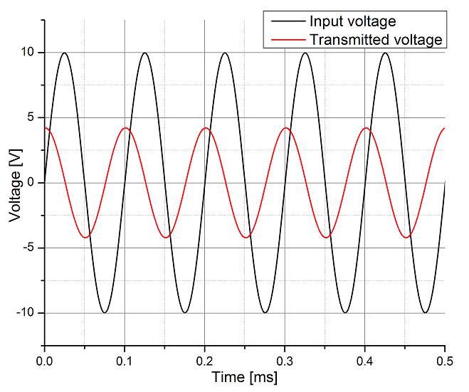
Transmitted voltage

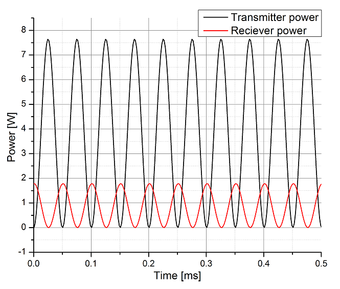
Transmitted power

The figures show that at a distance of 25 (cm) the transmitted voltage turned out to be approximately 2.5 less than the input, and the transmitted peak power was approximately 4 times less than the power consumed from the input, which is consistent with the formulas obtained .

In conclusion, we describe what measures can be taken to increase the transmitted power:

increase the number of turns in the coils $n_1, n_2$
increase the turn radius $a_1, a_2$
increase transmission frequency $f$
reduce the distance between the coils $d$
insert magnetic core belonging to both coils (closed or open)
enter an open magnetic core belonging only to the receiver coil

Perhaps writing this article imposes an obligation on the author to make and test such a system of two coils in the laboratory, but this is a completely different story. Thank you for attention.

Literature

Sivukhin, D.V. “General course of physics. Vol. 3: Electricity and magnetism. "(1990).
Bessonov, Lev Alekseevich. Theoretical foundations of electrical engineering. Electromagnetic field. Limited Liability Company Publishing Yurayte, 2012.
Lavrentyev, M. A., and B. V. Shabbat. "The theory of functions of a complex variable." (1972).

All Articles